Course Overview
Watch this welcome video from your instructor:
Course Description
Is this statement true? why?
The course will revolve heavily around this recurring question. Across different mathematical topics, students will be faced with new statements to grapple with, and the techniques needed to tackle them.
This aims to be a contextualized course. We will write code on occasion, and introduce high-level mathematical challenges in computer science.
This course will help you develop the ability to think logically and mathematically, with an emphasis on logical reasoning and communicating using mathematics. In the unit on logic and proofs, you'll learn to identify, evaluate, and make convincing mathematical arguments.
You'll review number systems, and their relevance to digital computers. You'll discuss and practice algebraic operations and concepts fundamental to Computer Science. The course also includes an introduction to counting and probability. You'll also explore how all of these methods are used in real-world computational problems.
Learning Outcomes
By the end of the course, you will be able to:
- Evaluate arguments, and identify the premises and conclusion of a mathematical argument
- Create diagrams to graphically depict the structure of an argument
- Decompose a given problem into smaller problems using recursion and induction
- Apply probability rules to determine the likelihood of an event
Instructor
- Santiago Camacho
- santiago.camacho@kibo.school
Please reach out by email with “[Mathematical Thinking]” in the subject, using your Kibo email address.
This course also has a Teaching Assistant, who will have their own office hours and who you can reach out to for additional assistance.
The Teaching Assistant and their contact information is:
- Oluwafemisire Ojuawo
- oluwafemisire.ojuawo@kibo.school
Live Class Time
Note: all times are shown in GMT.
- Thursdays at 3:00 PM - 4:30 PM GMT
The following week’s lessons will be released every Sunday.
Office Hours
- Instructor: Thursdays at 5:00 PM - 6:00 PM GMT
- Teaching Assistant: Fridays at 7:00 PM GMT to 8:00 PM GMT
Live Classes
Each week, you will have a live class (see course overview for time). You are required to attend the live class sessions.
Video recordings and resources for the class will be posted after the classes each week. If you have technical difficulties or are occasionally unable to attend the live class, please be sure to watch the recording as quickly as possible so that you do not fall behind.
| Week | Topic | Notes | Live Class Video | Practice Problems | Class Problems with Solutions | Additional Solutions |
|---|---|---|---|---|---|---|
| 1 | Elementary Functions | Notes | YouTube | Practice | Class Problems | Solutions |
| 2 | Propositional Logic | Notes | YouTube Part2 | Practice | Class Problems | Solutions |
| 3 | Sets | Notes | YouTube | Practice | Class Problems | Solutions |
| 4 | Proofs | Notes | YouTube | Practice | Class Problems | Solutions |
| 5 | Counting | Notes | YouTube | Practice | Class Problems | Solutions |
| 6 | Probability | Notes | YouTube | Practice | Class Problems | Solutions |
| 7 | Review | No Notes | YouTube | Practice | No Class Problems | No Problems |
| 8 | Functions and Relations | Notes | YouTube | Practice | Class Problems | Solutions |
| 9 | Number Theory | Notes | YouTube | Practice | No Class Problems | No Problems |
| 10 | Number Theory Part 2 | Notes | YouTube | Practice | Class Problems | Solutions |
If you miss a class, review the slides and recording of the class and submit the activity or exercise as required.
https://youtu.be/K7OFxhlKiPs
Assessments
Your overall course grade is composed of these weighted factors:
- Weekly Assignments: 63%
- Projects: 37%
Weekly Assignments
Each week you will be given an Assignment, where you'll practice the concepts covered in the readings and lessons. The assignments let you practice with the topics you cover that week, explore applications and connections, and check your own understanding of the material.
The assignments are completed within Gradescope, and they must be completed within two days of the live class session.
Practice Problems
In addition to the Gradescope Assignments, you are provided with practice problems in your Anchor course material. These practice problems sets are very valuable in that they will help you test your understanding of the material that you completed that week and ensure that you are ready to complete the assignment. It is highly recommended that you complete as many of the Practice Problems as possible.
Project
You will complete two projects during the term. You will be given additional time to complete the projects, and they will represent a significant portion of your final grade.
Getting Help
If you have any trouble understanding the concepts or stuck on a problem, we expect you to reach out for help!
Below are the different ways to get help in this class.
Discord Channel
The first place to go is always the course's help channel on Discord. Share your question there so that your Instructor and your peers can help as soon as we can. Peers should jump in and help answer questions (see the Getting and Giving Help sections for some guidelines).
Message your Instructor on Discord
If your question doesn't get resolved within 24 hours on Discord, you can reach out to your instructor directly via Discord DM or Email.
Office Hours
There will be weekly office hours with your Instructor and your TA. Please make use of them!
Tips on Asking Good Questions
Asking effective questions is a crucial skill for any computer science student. Here are some guidelines to help structure questions effectively:
-
Be Specific:
- Clearly state the problem or concept you're struggling with.
- Avoid vague or broad questions. The more specific you are, the easier it is for others to help.
-
Provide Context:
- Include relevant details about your environment, programming language, tools, and any error messages you're encountering.
- Explain what you're trying to achieve and any steps you've already taken to solve the problem.
-
Show Your Work:
- If your question involves code, provide a minimal, complete, verifiable, and reproducible example (a "MCVE") that demonstrates the issue.
- Highlight the specific lines or sections where you believe the problem lies.
-
Highlight Error Messages:
- If you're getting error messages, include them in your question. Understanding the error is often crucial to finding a solution.
-
Research First:
- Demonstrate that you've made an effort to solve the problem on your own. Share what you've found in your research and explain why it didn't fully solve your issue.
-
Use Clear Language:
- Clearly articulate your question. Avoid jargon or overly technical terms if you're unsure of their meaning.
- Proofread your question to ensure it's grammatically correct and easy to understand.
-
Be Patient and Respectful:
- Be patient while waiting for a response.
- Show gratitude when someone helps you, and be open to feedback.
-
Ask for Understanding, Not Just Solutions:
- Instead of just asking for the solution, try to understand the underlying concepts. This will help you learn and become more self-sufficient in problem-solving.
-
Provide Updates:
- If you make progress or find a solution on your own, share it with those who are helping you. It not only shows gratitude but also helps others who might have a similar issue.
Remember, effective communication is key to getting the help you need both in school and professionally. Following these guidelines will not only help you in receiving quality assistance but will also contribute to a positive and collaborative community experience.
Screenshots
It’s often helpful to include a screenshot with your question. Here’s how:
- Windows: press the Windows key + Print Screen key
- the screenshot will be saved to the Pictures > Screenshots folder
- alternatively: press the Windows key + Shift + S to open the snipping tool
- Mac: press the Command key + Shift key + 4
- it will save to your desktop, and show as a thumbnail
Giving Help
Providing help to peers in a way that fosters learning and collaboration while maintaining academic integrity is crucial. Here are some guidelines that a computer science university student can follow:
-
Understand University Policies: Familiarize yourself with Kibo's Academic Honesty and Integrity Policy. This policy is designed to protect the value of your degree, which is ultimately determined by the ability of our graduates to apply their knowledge and skills to develop high quality solutions to challenging problems--not their grades!
-
Encourage Independent Learning: Rather than giving direct answers, guide your peers to resources, references, or methodologies that can help them solve the problem on their own. Encourage them to understand the concepts rather than just finding the correct solution. Work through examples that are different from the assignments or practice problems provide in the course to demonstrate the concepts.
-
Collaborate, Don't Complete: Collaborate on ideas and concepts, but avoid completing assignments or projects for others. Provide suggestions, share insights, and discuss approaches without doing the work for them or showing your work to them.
-
Set Boundaries: Make it clear that you're willing to help with understanding concepts and problem-solving, but you won't assist in any activity that violates academic integrity policies.
-
Use Group Study Sessions: Participate in group study sessions where everyone can contribute and learn together. This way, ideas are shared, but each individual is responsible for their own understanding and work.
-
Be Mindful of Collaboration Tools: If using collaboration tools like version control systems or shared documents, make sure that contributions are clear and well-documented. Clearly delineate individual contributions to avoid confusion.
-
Refer to Resources: Direct your peers to relevant textbooks, online resources, or documentation. Learning to find and use resources is an essential skill, and guiding them toward these materials can be immensely helpful both in the moment and your career.
-
Ask Probing Questions: Instead of providing direct answers, ask questions that guide your peers to think critically about the problem. This helps them develop problem-solving skills.
-
Be Transparent: If you're unsure about the appropriateness of your assistance, it's better to seek guidance from professors or teaching assistants. Be transparent about the level of help you're providing.
-
Promote Honesty: Encourage your peers to take pride in their work and to be honest about the level of help they received. Acknowledging assistance is a key aspect of academic integrity.
Remember, the goal is to create an environment where students can learn from each other (after, we are better together) while we develop our individual skills and understanding of the subject matter.
Academic Integrity
When you turn in any work that is graded, you are representing that the work is your own. Copying work from another student or from an online resource (including generative AI tools like ChatGPT) and submitting it is plagiarism.
As a reminder of Kibo's academic honesty and integrity policy: Any student found to be committing academic misconduct will be subject to disciplinary action including dismissal.
Disciplinary action may include:
- Failing the assignment
- Failing the course
- Dismissal from Kibo
For more information about what counts as plagiarism and tips for working with integrity, review the "What is Plagiarism?" Video and Slides.
The full Kibo policy on Academic Honesty and Integrity Policy is available here.
Core Reading
The following materials were key references when this course was developed. Students are encouraged to use these materials to supplement their understanding or to diver deeper into course topics throughout the term.
- DeLancey, C. (2017). A Concise Introduction to Logic. Open SUNY Textbooks
- Cleave, M. (2016). Introduction to Logic and Critical Thinking
Supplemental Reading
This course references the following materials. Students are encouraged to use these materials to supplement their understanding or to diver deeper into course topics throughout the term.
- Devlin, K. (2012) Introduction to Mathematical Thinking.
- https://slim.computer/visual-proofs/proof/
Assignment 0
Complete the assignment on Gradescope using the link below.
After you have completed the assignment, export a PDF of the completed assignment and upload to Anchor below.
Elementary Functions
Throughout our education we have encountered several functions that turn up over and over throughout many math courses taken in the past, such as multiplication and addition.
These lessons are set to review a few of their properties.
You will be able to identify linear functions, affine functions, polynomials, exponentials and logarithms, as well as being able to manipulate them through the use of their specific properties.
Resources:
Number Sets
We will be discussing four important sets of numbers: natural numbers, integer numbers, rational numbers, and real numbers. In future weeks of the class we will dive deeper into the meaning, properties, and operations regarding general sets, but for the purpose of this section we can just think of a set as a collection of numbers.
Each of the following sets are traditionally represented with the double struck capital letters $\mathbb{N}, \mathbb{Z}, \mathbb{Q}, \mathbb{R}$ for natural numbers, integers, rational numbers and real numbers. We will give a few examples of their elements that encompass these sets.
Natural Numbers
We begin with natural numbers, which are the counting numbers we use to count objects. Depending on who you ask, Natural numbers start from 0 or from 1. Regardless they continue indefinitely. You should always make sure that you are in accord with the text, video, class or person that you are interacting with on whether or not you consider 0 to be part of the natural numbers.
For the purpose of this class the Natural Numbers start at 0. They are denoted by the symbol $\mathbb{N}={0, 1, 2, 3, 4, ...}$.
Integer Numbers
Building upon natural numbers, we introduce integers. Integers include all the natural numbers and their negatives. In other words, integers are positive and negative whole numbers, along with zero. We use the symbol $\mathbb{Z}={..., -3, -2, -1, 0, 1, 2, 3, ...}$ to represent the set of integers.
Rational Numbers
Next, we move on to rational numbers. Rational numbers are numbers that can be expressed as fractions, where the numerator and denominator are both integers. These numbers can be written in the form $p/q$, where $p$ and $q$ are integers, and $q$ is not equal to zero. Rational numbers include both terminating decimals and recurring decimals. Some examples of rational numbers are 1/2, -3/4, and 0.25. The set of rational numbers is denoted by the symbol $\mathbb{Q}$.
Real Numbers
Finally, we come to real numbers, which encompass all rational and irrational numbers. Real numbers are essentially the numbers we use in everyday life. They include fractions, decimals, and even numbers that cannot be expressed as fractions, such as the square root of 2 (√2) or pi (π). Real numbers are represented by the symbol $\mathbb{R}$.
Summary
Natural numbers ($\mathbb{N}$) are the counting numbers starting from 0.
Integer numbers ($\mathbb{Z}$) include natural numbers, and their negatives.
Rational numbers ($\mathbb{Q}$) are numbers that can be expressed as fractions.
Real numbers ($\mathbb{R}$) include both rational and irrational numbers.
Understanding these number systems is fundamental in mathematics and various other fields. They allow us to perform calculations, solve equations, measure quantities, and explore the vastness of mathematical concepts.
Section Video
Constant Functions
Key Ideas:
- Define constant functions
- Establish graphical properties of constant functions
A Simple example
Usually in programing we define some constants and give them a name. We can think of these as constant functions.
Constant functions in one variable
As its name suggests, a constant function is a function whose output is constant independent of the input. When we graph a constant function in one variable on the cartesian plane we obtain a horizontal line.
In applications constant functions usually correspond to some form of initial condition, such as the principal in an investment, or an initial cost of production.
Constant functions in two or more variables
When considering constants as functions of two variables we will see that their graph would correspond to just a horizontal plane that cuts the z-axis at the number that the constant represents.
References
Linear Functions
Key Ideas:
- Define linear functions
- Establish graphical properties of linear functions
Linear functions are used in several areas of knowledge, such as mathematics engineering and even the social sciences. Some concrete applications in computer science involve optimization, image processing, graph algorithms, quantum computing, cryptography, and machine learning just to name a few.
A simple example
You can easily calculate the expected pay of an hourly job as a function of the hours that were worked using a linear function. For example if you are paid $ $35 $ then your expected pay function would be
$EP(h) = 35 \cdot h$ where $h$ is the number of hours worked.
Linearity
A function $f$ is said to be linear if it satisfies the following two conditions
- $f(x + y) = f(x) + f(y)$ for all inputs $x, y$
- $f(a x) = a f(x)$ for all real numbers $a$
In the real numbers, linear functions on one variable are always going to have the form
- $f(x) = k x$ for some real number $k$.
In particular the function only depends on the value of $f(1)$. As indeed, if $x$ is a real number then $f(x)= x f(1)$.
Graphs of linear functions
The graph of every linear functions in one variable look like a line that goes through the origin. It is easy to graph this functions as you only need one value that is non-zero, and then just join the origin to the point corresponding to the (input,output) that you obtained.
When dealing with linear functions of two variables, their graphical representation will correspond to that of planes in the three dimensional space that cut through the origin.
Section Video
Affine Functions
Affine functions play a crucial role in mathematics and have many practical applications in various fields. Let's explore what affine functions are and how they are defined.
An affine function, also known as an affine transformation or an affine map, is a type of mathematical function that preserves lines and ratios of distances. In simpler terms, an affine function combines two essential components: a linear function and a translation.
A simple example
Modeling the cost of production of a certain number of units for your business is a function that depends on an initial cost and then an increased cost per additional unit. As such it can be modeled with the affine function
$C(u)= I + c u$ where $I$ is the initial cost of production, $c$ is the cost per individual unit produced, and $u$ is the number of units produced.
Definition
An affine function can be defined in the form:
- $f(x) = mx + b$,
where $f(x)$ represents the output value, $x$ is the input value, $m$ is the slope or gradient of the linear part of the function, and $b$ is the constant term or y-intercept that represents the translation.
Characteristics
Key characteristics of affine functions include:
-
Line Preservation: Affine functions preserve straight lines. If you plot points on a line, their images under an affine function will still form a line, although it may be shifted, scaled, or rotated.
-
Ratio Preservation: Affine functions maintain the ratio of distances along parallel lines. This property is particularly useful in geometric transformations and computer graphics.
-
Linear and Translation Components: Affine functions consist of both a linear component (represented by $mx$) and a translation component (represented by $b$). The linear component determines the slope or inclination of the function, while the translation component determines the vertical shift.
-
Affine Combinations: Affine functions can be combined through addition, subtraction, multiplication by scalars, and composition to form more complex transformations.
Affine functions find applications in various fields, including computer graphics, image processing, optimization, economics, and physics. They provide a flexible and efficient framework for modeling and solving real-world problems.
In summary, an affine function is a mathematical function that combines a linear component and a translation component. It preserves lines and ratios of distances, making it a powerful tool for a wide range of applications. Understanding affine functions is fundamental in mathematics and opens the door to exploring more advanced concepts in geometry, algebra, and beyond.
Section Video
Polynomials
Key Ideas
- Define monomials
- Define polynomials
- Define identify the degrees of monomials and polynomials.
- Define and identify the coefficients of a polynomial.
Interest
Sometimes we are interested in modeling or describing several events that do not behave directly like a line. Such as the height of a rollercoaster, the time complexity of several sorting algorithms, the height of a ball thrown in the air, just to mention a few.
In this section we will be able to identify polynomials, the jargon around them and a few of their properties.
Examples
The dish in a dish antenna follows the shape of the graph of a polynomial of second degree in two variables such as
$4x^2 + 4y^2$
Monomials
A monomial is a term composed of the product between one or more variables and a real number. For example, if $x, y,$ and $z$ are variables, then the following are monomials
-
$2x$
-
$3x^2$
-
$5xy$
-
$\pi x^3 y z^2$
-
$1$
The degree of a monomial is the sum of the exponents of its variables.
-
$2x$ has degree 1
-
$3x^2$ has degree 2
-
$5xy$ has degree 2
-
$\pi x^3 y z^2$ has degree 6
-
$1$ has degree 0
The number of variables of a monomial is the number of distinct variable symbols that appear.
-
$2x$ is a monomial on 1 variable.
-
$3x^2$ is a monomial on 1 variable.
-
$5xy$ is a monomial on 2 variables.
-
$\pi x^3 y z^2$ is a monomial on 3 variables.
-
$1$ has no variables.
The coefficient of a monomial is the number that multiplies the variables of the monomial.
Polynomials
A polynomial is a term composed by a sum of monomials. For example:
-
$2x +1$
-
$3x^3 +2x$
-
$x+2xy + z^2$
-
$1$
The degree of a polinomial is the highest degree of that of its monomials. For example:
-
$2x +1$ has degree 1
-
$3x^3 +2x$ has degree 3
-
$x+2xy + z^2$ has degree 2
-
$1$ has degree 0
The number of variables of a polynomial is the number of distinct variable symbols that appear in all of the terms. For example:
-
$2x +1$ has 1 variable
-
$3x^3 +2x$ has 1 variable
-
$x+2xy + z^2$ has 3 variables
-
$1$ has 0 variables
The coefficients of a polynomial are the list of all coefficients that appear in any of the monomials that add up to the polynomial.
-
$2x +1$ has 1,2 as its coefficients
-
$x+2xy + 3z^2$ has 1,2,3 as its coefficients
-
$1$ has 1 as its coefficient
When looking at a polynomial in one variable of degree $n$ that has less than $n+1$ monomials, we will consider 0 as a coefficient of the polynomial, as you may think of zero as the number multiplying $x^m$ where $m$ is smaller than n.
- We can say that $3x^3 +2x$ has 3,2,and 0 as its coefficients.
Again when dealing with polynomials with one variable we might also be interested in the order of the coefficients starting by the omes corresponding to monomials with the higher degrees.
- We can list the coefficients of $3x^3 +2x$ as (3,0,3,0).
The leading coefficient of a polynomial in one variable is the non-zero coefficient corresponding to the monomial with the highest degree. For example:
-
$2x +1$ has 2 as its leading coefficient.
-
$3x^3 +2x$ has 3 as its leading coefficient.
Graphs of Polynomials
In general graphs of polynomials are not easy to trace perfectly, unles you are familiar with some techniques from calculus, and further mathematical courses.
For polynomials in one variable there are some tendencies that you can obtain for the graph just from looking at the degree and the leading coefficient. In particular we will care mostly about the parity (whether it is odd or even) of the degree of the polynomial, and the sign (whether it is positive or negative) of the leading coefficient.
-
If the degree of the polynomial is even and the leading coefficient is positive then the shape will look like an upside cup
-
If the degree of the polynomial is even and the leading coefficient is negative, then the shape will look like a upside-down cup
-
If the degree of the polynomial is odd and the leading coefficient is positive then the graph is going to start at the negatives, cross the x-axis and continue to grow in the positives
-
If the degree of the polynomial is odd and the leading coefficient is negative then the graph is going to start at the negatives, cross the x-axis and continue to decrease in the negatives.
Video on Polynomials
Summation Notation
When convenient we will use the Sigma-summation notation to abbreviate sums. In general if you have a list of elements $x_1, x_2, ..., x_n$ and you want to express their sum, instead of writing the potentially ambiguous $x_1 + x_2 + ... + x_n$ we would write $\sum_{i=1}^{n}x_n$
The above sum is read fully as the "indexed sum by i from $i$ equal to 1 up to $i$ equal to $n$ of $x_i$", but we will abbreviate it as "the sum from $i = 1$ to $n$ of $x_i$".
Examples
Consider the sum of the first ten natural numbers.
- $\sum_{i=1}^{10} i=55$
Or a polynomial where the coefficients correspond to odd numbers.
- $\sum_{i=0}^{3}(2i+1)x^i = 1+3x+5x^2+7x^3$
Video on Summation
Product Notation
When convenient we will use the Pi-product notation to abbreviate products. In general if you have a list of elements $x_1, x_2, ..., x_n$ and you want to express their product, instead of writing the potentially ambiguous $x_1 \cdot x_2 \cdot ... \cdot x_n$ we would write $\prod_{i=1}^{n}x_n$
The above product is read fully as "the indexed product by i from $i$ equal to 1 up to $i$ equal to $n$ of $x_i$", but we will abbreviate it as "the product from $i = 1$ to $n$ of $x_i$".
Examples
-
Let $f$ be any function $\prod_{n=5}^{10}f(n)=f(5)f(6)f(7)f(8)f(9)f(10)$
-
$\prod_{i=1}^5 i = 120$
-
$\prod_{n=1}^{4}2^i = 1024$
Video on Products
Polynomial Roots and Factorization
Polynomials are essential mathematical expressions that appear in various areas of mathematics and science. Understanding their roots and factorization is key to solving equations, graphing functions, and analyzing polynomial behavior. Let's delve into these concepts!
Polynomial Roots
The roots of a polynomial are the values of the variable that make the polynomial equal to zero. In other words, if we substitute a root into the polynomial, the resulting value will be zero. These roots are also known as zeros, solutions, or x-intercepts of the polynomial. For example, consider the polynomial $f(x) = x^2 - 4x + 3$. To find its roots, we set $f(x)$ equal to zero: $x^2 - 4x + 3 = 0$ and solve for $x$.
By factoring or using the quadratic formula, we can find the roots of this polynomial: $x = 1$ and $x = 3$. These values make the polynomial equal to zero, so they are the roots of the equation.
Polynomial Factorization
Factorization involves breaking down a polynomial into a product of simpler polynomials. This process allows us to express a polynomial in a more manageable form and can help reveal its roots. For example, let's consider the polynomial $f(x) = x^2 - 4x + 3$ again. We can factor this polynomial as: $f(x) = (x - 1)(x - 3)$.
Here, we have expressed the polynomial as a product of two simpler polynomials, $(x - 1)$ and $(x - 3)$. These factors represent the linear terms associated with the roots of the original polynomial.
Factoring can be more complex for higher-degree polynomials. In such cases, techniques like synthetic division, long division, or factoring by grouping may be employed. Now a days you may also use a computer algebra system to obtain the factorization of polynomials.
By factoring a polynomial, we gain valuable insights into its behavior, such as its roots and more detailed information on the shape of its graph.
The Fundamental Theorem of Algebra:
The Fundamental Theorem of Algebra states that every polynomial equation with complex coefficients has at least one complex root. This theorem guarantees that we can always factorize a polynomial into a product of linear terms, that could potentially involve complex values. Now, we are focusing in this class mostly on real numbers. We do have that every polynomial with real roots can be factorized into a product of linear and quadratic terms with real coefficients.
By understanding polynomial roots and factorization, we can solve equations, graph polynomial functions, and analyze their behavior. These concepts have applications in algebra, calculus, physics, engineering, and many other fields.
Remember, finding roots and factorizing polynomials often requires practice and familiarity with different factoring techniques. Don't hesitate to explore more examples and solve polynomial equations to enhance your understanding.
Introduction to Exponential Functions
Introduction
Exponential functions play a fundamental role in mathematics and are widely used in various fields, including science, finance, and computer science. We will explore the basics of exponential functions, their properties, and how to work with them.
A simple example
When you have a binary tree structure, the number of leafs of the tree can be calculated with the function
$L(l)=2^l$ where $l$ is the number of levels of the tree.
Another example
If you are interested in learning what is the rate of growth of money deposited (loaned) with an interest rate of $r$ compounded annually then you can figure that out using the exponential function
$R(y)= (1+r)^y$ where $y$ is the number of years the money would be in the deposit.
What is an Exponential Function?
An exponential function is a mathematical function of the form $f(x) = a^x$, where $a$ is a positive constant and $x$ is a variable. The base $a$ is typically greater than 1, but it can also be a number between 0 and 1, excluding 0. The variable $x$ can be any real number or even a complex number. Even though many of the facts that we will expose also hold for exponentials with complex number values we will mainly focus on the variable taking real inputs.
Properties of Exponential Functions
Growth or Decay
Exponential functions can represent both growth and decay phenomena. When the base $a$ is greater than 1, the function exhibits exponential growth. Conversely, when 'a' is between 0 and 1, excluding 0, the function exhibits exponential decay.
Domain and Range
The domain of an exponential function is the set of all real numbers. The range depends on whether the function base is or is not 1. If the base of the exponential function is different than 1, then the range is all positive real numbers. If the base of the exponential function is 1, then the range is just the set ${1}$.
Continuous Growth
Exponential functions exhibit continuous growth or decay, meaning that they change gradually over time rather than in discrete steps.
Asymptote
Exponential functions have a horizontal asymptote, which is a line that the function approaches but never reaches. The asymptote is typically $y = 0$ for growth functions when approching $-\infty$ and $y = 0$ for decay functions when approching $(+)\infty$.
Additive property of Exponents
Probably the most important property of exponential functions, and in fact one of its defining characteristics, is that it opens up sums into products. Namely
- $f(x + y) = f(x) f(y) $
This property bears a lot of interesting facts about exponentials, including some of the following:
-
$f(0) = 1$ or $f(0) = 0$ but we will not deal with the $f(0)=0$ case since:
-
If $f(0) = 0$ then $f(x)= 0$ for all $x$
-
$f(-x) = \frac{1}{f(x)}$
Common Applications:
Exponential functions have numerous applications in various fields. Some common applications include:
- Population growth and decay
- Compound interest and investments
- Radioactive decay
- Biological processes
- Epidemic modeling
- Electronics and signal processing
Video on Exponentials
Introduction to Logarithmic Functions
Introduction
Logarithmic functions, or logarithms for short, are essential mathematical tools that arise from the study of exponential functions. They provide a way to solve equations involving exponential relationships, convert between different bases, and analyze the behavior of various phenomena. In this lesson, we will explore the basics of logarithmic functions, their properties, and their applications.
What is a Logarithmic Function?
A logarithmic function is the inverse of an exponential function. It represents the relationship between a given base and its exponent. The general form of a logarithmic function is written as $f(x) = log(base, x)$, where 'base' is a positive number greater than 1, and 'x' is the input value.
Application
Let us assume that you are investing some capital on an account that provides a $5\%$ interest rate compounded annually If you wanted to find out when would your money achieve a certain percentage growth you would use a logarithmic function
$Y(p) = \log(1+5% ,p)$ where $p$ is the percentage growth that you are looking for (e.g %200 when wanting to figure out when your money would double).
Properties of Logarithmic Functions:
Domain and Range
The domain of a logarithmic function is the set of all positive real numbers. The range depends on the base and is typically the set of all real numbers.
Inverse of Exponential Functions
Logarithmic functions and exponential functions are inverses of each other. If $y = a^x$, then $x = log(base, y)$, where the base s the same in both the exponential and logarithmic functions.
Logarithmic Identities:
-
$log(base, 1) = 0$ The logarithm of 1 to any base is always 0.
-
$log(base, base) = 1$ The logarithm of the base to the same base is always 1.
Logarithmic Laws
-
Product Rule: $log(base, x * y) = log(base, x) + log(base, y)$
-
Quotient Rule: $log(base, x / y) = log(base, x) - log(base, y)$
-
Power Rule: $log(base, x^a) = a * log(base, x)$
Fields of application
Logarithmic functions find applications in various fields. Some common applications include:
-
Computing pH levels in chemistry
-
Measuring sound intensity with decibels
-
Evaluating earthquake intensity using the Richter scale
-
Analyzing population growth and decay models
-
Studying the behavior of radioactive decay
-
Solving exponential equations
Logarithmic functions provide a powerful tool for solving exponential equations, understanding exponential relationships, and analyzing various phenomena. As you delve deeper into logarithmic functions, you will encounter more advanced concepts and applications. Remember to practice and explore further to strengthen your understanding.
Resources
Problem Set 0
Submission
- You may collaborate and are encouraged to collaborate with your peers. If you do, be sure to understand the material and write it out in your own words.
There is no requirement to submit the material, but this will help you solidify the concepts.
Problems
-
Determine which sets of numbers do the following numbers belong to amon Naturals $ \mathbb{N} $, Integers $ \mathbb{Z} $, Rationals $ \mathbb{Q} $ , and Reals $ \mathbb{R} $. Select all that apply.
a. 25
b. 32.5
c. 1/3
d. π/3
-
Determine which kind of function is represented by the following expression on $x$.
a. 35
b. $2x$
c. $2x +5$
d. $x^{2} + 3x -1$
e. $2^{x}$
f. $\log(x) - \log(2x)$
-
Solve the following systems of equations.
a. $x-y = -1$ and $3x = 3(y+2)$
b. $x-y = -1$ and $3x = y+3$
-
Factor the following polynomials
a. $9 + 12x + 4x^{2}$
b. $25 + 20x + 4 x^{2}$
c. $25 - 20x + 4 x^{2}$
d. $9x^2 - 243$
-
Compute the following values.
a. $\log_{10}(10000)$
b. $\log_{2}(8) - \log_{2}(32)$
c. $\log_{2}(1/16)$
-
Find the values of x that satisfy the equations below.
a. $\log_{2}(x) + \log_4(x) = 3$
b. $4^{x} - 2^{x+1} = 0$
c. $10^{2x+2} = 50^{x+1}$
Assignment 1
Complete the assignment on Gradescope using the link below.
After you have completed the assignment, export a PDF of the completed assignment and upload to Anchor below.
Propositional Logic
How do we know if an argument is sound? What are the rules around what kinds of statements we can make?
These lessons are focused on propositional logic: the rules that govern logical statements. You'll learn the mathematical notation for these rules, and start to formalize logical statements you are used to making in your life when you speak.
You'll also practice evaluating chains of reasoning to verify that the reasoning is correct, or, if it's mistaken, locating which steps are invalid.
Resources:
- A Concise introduction to logic part 1
- Discrete mathematics - an open introduction part 3.1
- Instructor reading for Propositional Logic
Propositional Logic
Key ideas:
- Defining what a proposition is.
- Recognizing ambiguous and unambiguous statements
- Recognizing atomic components of a sentence
- Establishing the goal of propositional logic
Building a clear language:
This may come as a surprise to some of you, but computers are not very smart at all! Sure, they can compute a lot of numbers, and we have been able to build incredible software to run on them. They are incredible machines, but at a fundamental level, all they do is follow instructions. There is no room for interpretation, they can't inherently ask follow up questions, or interpret the instructions you provide them in different way. Computers follow instructions literally.
As you will see in your practice of programming, this means that translating the way you think into something computers understand can be tricky. One of the key goals we will have in how we think about programs is unambiguity: There should be only one possible way to interpret what we say.
Propositions:
For the purposes of this course, a proposition is simply a sentence. However, we want to focus ourselves and think through sentences that are unambiguous. This means we should be able to evaluate all our sentences, all our propositions, as being either True or False.
Let's look at some pairs of sentences and see if they are propositions or not:
Tobi is kind of tall.
Tobi is 1.6 meters tall.
The first sentence is subjective! some may find Tobi tall, some may not. What's considered tall in a given area may not be in another. The second sentence however is verifiable: We can measure Tobi and say if the sentence is True or False.
This song is bad!
This song is in English
The second sentence is straightforward to verify: We can look at the lyrics and tell if the song is in English or not. The first sentence is not only ambiguous - you might like the song, and I might not - but the word "bad" is sometimes used to actually indicate the complete opposite in slang! The word itself is now ambiguous.
Someimes, we will have to grapple with challenging sentences that are impossible to evaluate for other reasons. Let's look at these last two examples:
This sentence is True.
This sentence is False.
Can the first sentence be True? well yes, it says so! Some propositions may have a unique value, either True or False, based on how they are crafted. They remain propositions nevertheless.
How about the second sentence then? Do you think it is a proposition? Think aboutit for a second before seeing the answer below
Well if it is a proposition, then it can be evaluated as either True or False:
- If we say that it is True, then that means the sentence is False, which is a contradiction!
- If we say that it is False, then that means the sentence is not False, so it is True! this is another contradiction!
This is inherently ambiguous: In the language we want to build, a proposition can not be both True and False at the same time, so we won't consider sentences like this.
Notation:
We will often assign a propositon to a variable $P$ instead of rewriting the whole sentence. Here $P$ simply stands for Proposition.
If we deal with multiple propositions, we carry on in alphabetical order, so our second proposition is $Q$, then $R$, etc.
Programming 1 connection:
In programming 1 you encountered boolean variables - variables that can either be True or False. You can effectively apply everything we learn about propositions in this course to boolean variables in programming!
Atomic sentences
Another big word! The concept behind atomic sentences is however simple. An atomic proposition is one that can not be broken down into connected propositions
Let's look at an example of an atomic sentence:
2 + 2 = 4
Is this a proposition? Yes! it is True that 2+2 is equal to 4.
Is there any way to "chop up" this proposition so that we find another proposition? Let's see:
- Can "2+2" evaluate to True or False? no, this sentence evaluate to 4 as we saw above.
- How about just "4"? 4 is neither True nor False, so it's not a proposition.
- How about "2 = 4"? Well this is a proposition - a False one. Does that mean that "2+2=4" is not atomic? well let's look at what's left of the initial sentence: "2 +": This is clearly not a proposition.
You can keep trying to break the sentence above into components, but you won't find a way to break it down into multiple propositions.
How about this sentence though?
If the DJ is playing Jerusalema, then Zainab is not on the dancefloor
Is "The DJ is playing Jerusalema" a proposition? sure is, the song is either playing or not.
How about "Zainab is not on the dancefloor" ? This is also a proposition, Zainab is either on the dancefloor or not.
So we can consider two different propositions here:
- $P$: The DJ is playing Jerusalema
- $Q$: Zainab is not on the dancefloor
Which makes our initial sentence take the form of if $P$, then $Q$
So our intiial sentence is not atomic. At the end of the day, this is good! this means we can combine simple, atomic propositions to express much larger and complex ideas. In the next sections we will cover the connectors we have to make complex propositions.
Section Video
References:
For further details, you can read through the following chapters:
Connectors part 1: And/Or:
Key ideas:
- Introduce the concept of truth tables.
- Introduce the truth table and notation for And.
- Introduce the truth table and notation for Or.
And:
The first connector we will discuss is AND. We use it often to connect propositions - "I am tired AND I am happy" - but let's formalize our understanding of it. First, in propositional logic, we often use a specific symbol to indicate AND rather than writin the word over and over again. The symbol for AND is $ \land $. So you should be able to interpret I am tired $ \land $ I am happy the same way as the above sentence.
Let $ P$, $ Q$ be two propositions. Instinctively, we have a sense for what $ P \land Q$ mean, but let's formalize it! remember that our key objective is to be very specific. This might be easier to reason about with concrete examples so:
- Let $ P$ be the proposition "You are reading this on your phone"
- Let $ Q$ be the proposition "You are listening to music"
How many scenarios do we have to consider? Well P can be either True or False, so that's two different values. Same for Q. So all together we have 4 scenarios:
- Both P, Q are True. $ P \land Q$ is therefore True
- P is True and Q is False. $ P \land Q$ is False
- P is False and Q is True. $ P \land Q$ is False
- Both P, Q are False. $ P \land Q$ is False
We will typically condense this information in what is called as a truth table:
| $ P$ | $ Q$ | $ P \land Q$ |
|---|---|---|
| True | True | True |
| True | False | False |
| False | True | False |
| False | False | False |
So to summarize, $ P \land Q$ is only True if and only if both $ P$ and $ Q$ are True.
Or:
- Let $ P$ be the proposition "You are reading this on your phone"
- Let $ Q$ be the proposition "You are reading this on your computer"
Let's jump straight ahead and define our symbol for Or to be $\lor$. So expressing "you are reading this on your phone or your computer" can be condensed to the proposition $ P \lor Q$.
We build up our truth table:
| $ P$ | $ Q$ | $ P \lor Q$ |
|---|---|---|
| True | True | True |
| True | False | True |
| False | True | True |
| False | False | False |
Priority:
Let's consider the following proposition: $ P \land Q \lor R$. How would we interpret this?
Well we know that $ P \land Q$ is a proposition, so we could evaluate it first, then combine it with the remaining $\lor R$ part.
But similarly, $ Q \lor R$ is also a valid proposition we could evaluate first. How do we prioritize?
By default, we note that $\land$ has a higher priority than $\lor$. This means that the first interpretation above is the correct and expected one. This is similar to basic algebra: If you see the expression 2 x 3 + 1 you should evaluate it as 7, not 8, as multipication has a higer priority. If you wanted to make sure the addition happened first, you could use parenthesis to indicate it. so 2 x (3 + 1) is equal to 8
You can similarly use parenthesis in propositional logic. So we have that:
- $ P \land Q \lor R$ is equivalent to $( P \land Q) \lor R$ since $\land$ has higher priority.
- $ P \land ( Q \lor R)$ is a different proposition altogether, as now prioritize the $\lor$
but don't take my word for it. Let's show this using truth tables. Two statements are equivalent if their respective truth tables are the same. Let's take a moment and fill up the table below and see if our statements are the same or different. Give it a shot for a few minutes before consulting the answer.
| $ P$ | $ Q$ | $ R$ | $ P \land Q \lor R$ | $ P \land ( Q \lor R)$ |
|---|---|---|---|---|
| True | True | True | ||
| True | True | False | ||
| True | False | True | ||
| True | False | False | ||
| False | True | True | ||
| False | True | False | ||
| False | False | True | ||
| False | False | False |
What you should see is that the fourth and fifth columns are different, so the two statements are not equivalent. You can use truth tables to assess if two propositions are the same by simply showing that they evaluate the same way in a table. Make sure to fill it up entirely before looking at the solution below.
| $ P$ | $ Q$ | $ R$ | $ P \land Q \lor R$ | $ P \land ( Q \lor R)$ |
|---|---|---|---|---|
| True | True | True | True | True |
| True | True | False | True | True |
| True | False | True | True | True |
| True | False | False | False | False |
| False | True | True | True | False |
| False | True | False | False | False |
| False | False | True | True | False |
| False | False | False | False | False |
We will continue looking at connectors in the next section.
Video on Conjunction Disjunction and Negation
References:
For further details, you can read through the following chapters:
- A Concise introduction to logic part 1.5 and 1.7
- Discrete mathematics - an open introduction part 0.2
Connectors part 2: Implication and Negation
Key ideas:
- Introduce the truth table and notation for implications
- Show De Morgan's law
Negation
This is the most straightforward connector. $\lnot$, also known as the NOT operator, simply changes the value of a proposition to its opposite. For example if we have $ P$: Zainab is on the dancefloor, then $\lnot P$ is the proposition Zainab is not on the dancefloor. This leads to the very straightforward Truth table:
| $ P$ | $\lnot P$ |
|---|---|
| True | False |
| False | True |
Negating complex propositions
As easy as it is to apply $\lnot$ to a single proposition, how do we apply it to more complex ones where other operators are involved? well, let's set up our initial truth table.
| $ P$ | $ Q$ | $ P \land Q$ | $\lnot(P \land Q)$ |
|---|---|---|---|
| True | True | True | False |
| True | False | False | True |
| False | True | False | True |
| False | False | False | True |
The above follows the simple rules we've established so far, but is there a way to simplify that proposition? Let's think about it with an example:
- Let $P$ be the proposition "The learner finished the problem set"
- and Let $Q$ be the proposition "The learner is taking a nap"
When we say $\lnot(P \land Q)$, we mean that it is not the case that the learner finished the problem set and that the learner is taking a nap. This means that at least one of the two propositions within must be False. This is in line with what we saw in the truth table above. At least one of the two propositions being false means that $P$ is false or $Q$ is false. Let's explore the new truth table below:
| $ P$ | $ Q$ | $ \lnot P$ | $\lnot Q$ | $ (\lnot P \lor \lnot Q)$ |
|---|---|---|---|---|
| True | True | False | False | False |
| True | False | False | True | True |
| False | True | True | False | True |
| False | False | True | True | True |
Notice that the last column of this truth table looks exactly the same as the last column of the prior one, leading us to state that $\lnot(P \land Q)$ and $ (\lnot P \lor \lnot Q)$ are equivalent
This is refered to De Morgan's law, and will be very handy for us throughout the rest of the term. Note that this also applies the other way around:
$\lnot(P \lor Q)$ and $ (\lnot P \land \lnot Q)$ are equivalent. Can you convince yourself that it is the case?
These two equivalences
$\lnot(P \lor Q)$ equivalent to $ (\lnot P \land \lnot Q)$
$\lnot(P \land Q)$ and $ (\lnot P \lor \lnot Q)$
are called De Morgan's Laws
Priority:
$\lnot$ has the highest priority of all operations we will cover, so it will be evaluated before anything else.
References:
For further details, you can read through the following chapters:
Connectors part 2: Implication and Negation
Key ideas:
- Introduce the truth table and notation for implications
- Define inverse, converse, and contrapositive.
Implications:
This is one of the more natural sentences for us to consider. If this, then that! This kind or proposition is often refered to as an implication. Let's consider one we've seen before:
If the DJ is playing Jerusalema, then Zainab is not on the dancefloor
Let $ P$ be "The DJ is playing Jerusalema". In the context of implications, this first proposition is refered to as the hypothesis Let $ Q$ be "Zainab is not on the dancefloor". In the context of implications, the proposition that occurs after the hypothesis is the conclusion
We can denote the same sentence above now with the shorthand. $ P \to Q$.
Let's try to build up our truth table. This one is not as straighforward so we will do it step by step.
| $ P$ | $ Q$ | $ P \to Q$ |
|---|---|---|
| True | True | |
| True | False | |
| False | True | |
| False | False |
If $ P$ is True, and $ Q$ is true, that means the DJ is playing Jerusalema, and Zainab is not the dancefloor. This is in line with our implication, so we should consider the implication True in this case.
What about the second scenario? The DJ is playing Jerusalema, but Zainab is still on the dancefloor! This situation contradicts our implication, so if that's the case, our implication is false.
| $ P$ | $ Q$ | $ P \to Q$ |
|---|---|---|
| True | True | True |
| True | False | False |
| False | True | |
| False | False |
Let's look at our third scenario: The DJ is not playing Jerusalema, and Zainab is not on the dancefloor. How does this information influence our assessment of the initial implication? Think about it for a few moments before proceeding.
I would argue that in this case, our implication remains True. This scenario gives us no infromation that invalidate it. Let's look at another example to emphasize this.
- Let $ R$: x is a multiple of 4
- Let $ S$: x is a multiple of 2
Consider $ R \to S$ - or in other words if x is a multiple of 4, then x is a multiple of 2. Intuitively, we know this to be True (although we can formally prove statements like this in a few weeks!)
So what about a scenario where x is equal to 6? In this case $ R$ is False, 6 is not a multiple of 4. However, $ S$ is True, as 6 is an even number. Is this a valid reason to no longer think that our implication is True? it isn't!
So we can update our truth table
| $ P$ | $ Q$ | $ P \to Q$ |
|---|---|---|
| True | True | True |
| True | False | False |
| False | True | True |
| False | False |
Similarly, we can conclude that the final scenario should also evaluate to True. Consider the scenario where x is 5. $ R$ and $ S$ are both False, but does that change anything to the truth of our initial statement $ R \implies S$ ? It does not! So to conclude our truth table for implications is
| $ P$ | $ Q$ | $ P \to Q$ |
|---|---|---|
| True | True | True |
| True | False | False |
| False | True | True |
| False | False | True |
This may seem counterintuitive to you at a glance. The key idea here is not to consider implications as more strict than they are: They simply say that the conclusion will always follow the hypothesis, but there may be other scenarios where the conclusion is True. The only way an implication is false is by showing that the hypothesis is True and the conclusion is False
We will look at some more strict connectors than implication in the next few sections. For now though, let's move on to a very simple one.
Converse, Inverse, Contrapositive
Given an implication $ P \to Q$, we can derive 3 related propositions:
1- The converse of our implication is $ Q \to P$ - Our initial hypothesis and conclusion swap.
2- The inverse of our implication is $\lnot P \to \lnot Q$ - if they hypothesis is not true then the conclusion is not true.
3- The contrapositive of our implication is $\lnot Q \to \lnot P$ - if the conclusion is not true, then the hypothesis is not true.
Let's find the converse, inverse, and contrapositive of our first implication: "If the DJ is playing Jerusalema, then Zainab is not on the dancefloor "
- The converse is: If Zainab is not on the dancefloor, then the dj is playing Jerusalema.
- The inverse is: If the dj is not playing Jerusalema, then Zainab is on the dancefloor.
- The contrapositive is: If Zainab is on the dancefloor, then the dj is not playing Jerusalema.
Let's build up the truth tables for each of these new propositions. Try it yourself before seeing the answer below:
| $ P$ | $ Q$ | $ P \to Q$ | $ Q \to P$ | $\lnot P \to \lnot Q$ | $\lnot Q \to \lnot P$ |
|---|---|---|---|---|---|
| True | True | True | True | True | True |
| True | False | False | True | True | False |
| False | True | True | False | False | True |
| False | False | True | True | True | True |
What do you notice? Which of these forms are equivalent to each other? Your tables should indicate that the inverse and conerse are equivalent, and that an implication and its contrapositive are equivalent. We will use this fact next week!
Priority:
$\to$ has the lowest priority, so $\land$ and $\lor$ will always be evaluated before it, unless parenthesis change that. $\lnot$ has the highest priority, so it will be evaluated before anything else.
VIdeo on implication and biconditional
References:
For further details, you can read through the following chapters:
Connectors part 3: If and Only If
Key Ideas:
- Defining if and only if in terms of an implication and its converse
- Defining the truth table of if and only if relationships
Biconditionals:
Intuitively, we should see that the two following propositions have a different meaning:
- If the DJ is playing Jerusalema, then Zainab is not on the dancefloor
- If and only if the DJ is playing Jerusalema, then Zainab is not on the dancefloor
Adding the only if wording doesn't only make the sentence sound more dramatic, it changes it makes it more strict: The only means that no other song will prevent Zainab from being on the dancefloor. She won't stop if she's tired. The only way Zainab is not on the dancefloor is if, and only if, the DJ plays Jerusalema.
This is stricter than the simple implication. In fact, another way to reason about "if and only if" - also known as biconditional statements - is that they are true when an implication and its converse are true
Let's consider the following truth table:
| $ P$ | $ Q$ | $ P \to Q$ | $ Q \to P$ | $( P \to Q) \land ( Q \to P)$ |
|---|---|---|---|---|
| True | True | True | True | True |
| True | False | False | True | False |
| False | True | True | False | False |
| False | False | True | True | True |
Thinking through this in english we have:
- An implication: If the DJ is playing Jerusalema, then Zainab is not on the dancefloor
- Its converse: If Zainab is not on the dancefloor, then the DJ is playing Jerusalema
When both are true, we can say that "If and only if the DJ is playing Jerusalema, then Zainab is not on the dancefloor". This is why we call this kind of statement "biconditional", as they are the combination of two "conditional" statements.
Let's simplify our truth table and introduce the formal statement for biconditionals: $\iff$
| $ P$ | $ Q$ | $ P \iff Q$ |
|---|---|---|
| True | True | True |
| True | False | False |
| False | True | False |
| False | False | True |
Priority
$\iff$ shares the same priority as $\to$
We have covered all our connectors now! so our final priority order is: 1- $\lnot$ 2- $\land$ 3- $\lor$ 4- $\to , \iff$
Video on Equivalent Propositions
References:
For further details, you can read through the following chapters:
Practice Problems Week 2
- You may collaborate and are encouraged to collaborate with your peers. If you do, be sure to understand the material and write it out in your own words.
There is no requirement to submit the material, but this will help you solidify the concepts.
Problems
-
Make a truth table for the statement $\neg P \to (Q \wedge R)$
-
Are the statements $P \to (Q\vee R)$ and $ (P \to Q) \vee (P \to R) $ logically equivalent?
-
Use De Morgan's Laws, and any other logical equivalence facts you know to simplify the following statements. Show all your steps. Your final statements should have negations only appear directly next to the sentence variables or predicates ($P$, $Q$,$E(x)$, etc.), and no double negations. It would be a good idea to use only conjunctions, disjunctions, and negations.
a. $ \neg((\neg P \wedge Q) \vee \neg(R \vee \neg S)) $
b. $ \neg((\neg P \to \neg Q) \wedge (\neg Q \to R)) $ (careful with the implications).
c. For both parts above, verify your answers are correct using truth tables. That is, use a truth table to check that the given statement and your proposed simplification are actually logically equivalent.
-
Consider the statement, “If a number is triangular or square, then it is not prime”
a. Make a truth table for the statement $(T \vee S) \to \neg P$.
b. If you believed the statement was false, what properties would a counterexample need to possess? Explain by referencing your truth table.
c. If the statement were true, what could you conclude about the number 5657, which is definitely prime? Again, explain using the truth table.
-
Tommy Flanagan was telling you what he ate yesterday afternoon. He tells you, “I had either popcorn or raisins. Also, if I had cucumber sandwiches, then I had soda. But I didn't drink soda or tea.” Of course you know that Tommy is the worlds worst liar, and everything he says is false. What did Tommy eat?
Justify your answer by writing all of Tommy's statements using sentence variables ($P$, $Q$, $R$, $S$, $T$), taking their negations, and using these to deduce what Tommy actually ate.
Hint: Write down three statements, and then take the negation of each (since he is a liar). You should find that Tommy ate one item and drank one item. ($Q$ is for cucumber sandwiches.)
-
Consider the following four cards in the figure. Each card has a letter on one side, and a shape on the other side.
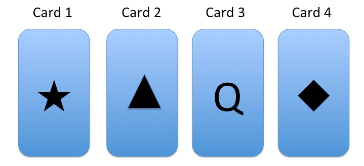
For each of the following claims, determine (1) the minimum number of cards you must turn over to check the claim, and (2) what those cards are, in order to determine if the claim is true of all four cards.
a. If there is a $P$ or $Q$ on the letter side of the card, then there is a diamond on the shape side of the card.
b. If there is a $Q$ on the letter side of the card, then there is either a diamond or a star on the shape side of the card.
-
Translate the following passage into our propositional logic. Prove the argument is valid.
Either Dr. Kronecker or Bishop Berkeley killed Colonel Cardinality. If Dr. Kronecker killed Colonel Cardinality, then Dr. Kronecker was in the kitchen. If Bishop Berkeley killed Colonel Cardinality, then he was in the drawing room. If Bishop Berkeley was in the drawing room, then he was wearing boots. But Bishop Berkeley was not wearing boots. So, Dr. Kronecker killed the Colonel.
-
Prove whether or not each of the following arguments is valid.
a. Premises: $((P \wedge Q) \iff R), (P \iff S), (S \wedge Q)$. Conclusion: $R$.
b. Premises: $(P \iff Q)$. Conclusion: $((P \to Q) \wedge (Q \to P))$.
c. Premises: $P, \neg Q$. Conclusion: $\neg(P \iff Q)$.
d. Premises: $( \neg P \vee Q), (P\vee \neg Q)$. Conclusion: $(P \iff Q)$.
e. Premises: $(P \iff Q), (R \iff S)$. Conclusion: $((P \wedge R) \iff (Q \wedge S))$.
f. Premises: $((P \vee Q) \iff R), (\neg P \iff Q)$. Conclusion: $R$.
g. Conclusion: $((P \iff Q) \iff (\neg P \iff \neg Q))$
h. Conclusion: $((P \to Q) \iff (\neg P \vee Q))$
References
These problems were drawn from:
Assignment 2
Complete the assignment on Gradescope using the link below.
After you have completed the assignment, export a PDF of the completed assignment and upload to Anchor below.
Sets
This week will focus on sets. Sets let mathematicians describe lots of things in the real world. When you know what kinds of operations you can do with sets, and what kinds of properties hold true, you can then apply those operations and properties to tons of specific situations and questions.
Resources:
- Section B1 from Introduction to Algorithms, Third edition.
- Discrete Mathematics: An open textbook section 0.3
- Set Theory and Proofs for Engineering Education, : 2019
- Instructor Reading for Sets
Guiding Question Week 3
Let's go through a little exercise thought exercise:
- Take a piece of paper and write the names of 10 people you know. Spread them around the page.
- Now, try to draw a line around the names of all the people who:
- You think can prepare a nice meal.
- You had a party with before?
- You can beat in a race.
- Did you end up with any of these categories being empty? Did you end up with anyone in all three categories?
Sets
Key Ideas:
- Define sets, as well as set builder notation.
- Introduce the concept of elements belonging to a set.
- Define established sets
- Introduce Cardinality and Complements of sets
What is a set?
Sets are a crucial but simple concept for our studies. A set is an unordered collection of objects. You can probably think of a few things that are sets: The set of all the players to ever play for Arsenal, or the set of meals you've tried in a given restaurant. The fundamental question we ask about sets is whether or not an item belongs to them. It does not matter what order it is within the set, just whether or not it is in it.
Let's talk notation with a simple set: let $ V = \{a, e, i, o, u, y\}$ be the set of all vowels. We can say that a belongs to the set $ V$, and that z does not belong to $ V$. We have notation for that too:
- $a \in V$ - in other words a belongs to the set $ V$, which is a True proposition
- $z \notin V$ - in other words z does not belongs to the set $ V$, which is also a True proposition
Finally, one thing to bear in mind is that sets can contain anything and everything: numbers, symbols, words, other sets.
For example consider: $ A = \{42, guide, \{79, 80, 82\}\}$ This set contains the number 42, the word guide, and the set {79, 80, 82}. This means that 80 $\notin A$, even though 80 belongs to a set within $ A$, it is not directly an element of $ A$
Programming 1 connection:
Sets are so useful, they are a core part of many programming languages as well. You can even create them in a similar fashion: In python you can recreate our set of vowels as follows:
v = {'a', 'e', 'i', 'o', 'u', 'y'}
You can view more information about sets in python here. Effectively everything we cover in this week's content can be done in code as well, so feel free to experiment with Python alongside this week's content!
Cardinality and the empty set:
Here we are again with new names, but cardinality is a simple concept: It refers to the size of a set. Our set of vowels $ V$ has 6 elements within it, so we can say that its cardinality is 6, or using a new symbol: |$ V$| = 6
Could there be a set with no elements at all? a cardinality of 0? well yes, we call it the empty set, and will use it extensively soon! We use it so often in fact that it gets its own symbol, $\emptyset$
Complements of sets:
If a set defines a specific collections that belong to it, then there surely is a set of elements who do not belong to it. We call that new set the complement. For example, we may think that the complement of $V$ is the set of all consonants. This makes intuitive sense, but there is a wrinkle here. $\bar V$, the complement of $V$, is the set of all elements which do not belong to $V$. Does the number 187 belong to $V$? it does not, so it should then belong to $\bar V$.
Let's combine the last two concepts we've encountered: What is the complement of the emptyset, $\bar \emptyset$? Well nothing is in the empty set, so everything should be in its complement. We refer to the set that contains everything as the Universal set, with symbol $U$
Famous sets
In the days and weeks to come, we will reason about specific groups of numbers. These are so commonly used that they have some shorthands we share here for reference:
- $\mathbb N$ is the set of natural number, or non-negative integers. Sometimes refered to as whole numbers, $\mathbb N = \{0, 1, 2, 3 ...\}$
- $\mathbb Z$ is the set of integers, this includes positive and negative whole numbers, $\mathbb Z = \{..., -2, -1, 0, 1, 2, ...\}$
- $\mathbb Q$ is the set of rational numbers, this includes all elements of $\mathbb Z$, as well as all numbers that can be expressed as finite fractions like 0.25, or 0.11
- $\mathbb R$ is the set of real numbers, this includes all elements of $\mathbb Q$, as well as all numbers that can not be expressed as finite fractions such as pi, or $\frac {1}{3}$
Set builder notation
Our initial examples of sets were quite small, so we could list all the elements directly, but as we saw in the famous sets above, some sets have infinitely many elements!
We can express the key idea behind a set using set builder notation, a shorthand that captures the conditions we set on an element to belong to a set. Let's try to define an infinite set: $E$ is the set of even, positive integers.
In other words, $E$ is the set of all elements of $\mathbb N$ that are even. so if we consider a variable $x \in E \to (x \in \mathbb N \land x$ is even $)$
We can further condense this idea by saying: $E = \{x \in \mathbb N : x\text{ is even }\}$. Here, the : is a shorthand for "such that". Following the : you can define propositions that must be true for all elements of the set.
There may be a few different ways to express a given definition of a set, but this is a helpful notation we should practice. Try to interpret the following four sets in plain english:
$\{x \in \mathbb R: x + 3 \in \mathbb N\}$
This is the set of all numbers x such that x + 3 is in $\mathbb N$, in other words a postive integer. In other words, this is the set {-3, -2, -1, 0, 1, ...} as -3 + 3 = 0 which belongs to $\mathbb N$
$\{x \in \mathbb N : x + 3 \in \mathbb N\}$ This is the set of all positive integers x such that x+3 is a positive integer. We end up with the set of positive integers $\mathbb N$
$\{x \in \mathbb R: x \in \mathbb N \lor -x \in \mathbb N\}$ This is the set of all numbers x such that x is a positive integer, or -x is a positive integer. If -x is a positive integer, then x is a negative integer. This ends up being a convoluted way to represent $\mathbb Z$, the set of all integers.
$\{x \in \mathbb R: x \in \mathbb N \land -x \in \mathbb N\}$ This is the set of all numbers x such that x is a positive integer, and -x is a positive integer. This is an odd combination, but there is one number which satisfies it: 0. This makes our answer the set {0}
Section Video
Next, we cover operations between sets.
References:
For further details, you can read through the following chapter:
Set Operations
Key Ideas:
- Introducing basic operations on sets: Union, Intersection, Substraction
Manipulating sets:
The same way we can combine numbers through addition, substractions, etc. There are a number of questions we may want to ask about multiple sets.
Union:
The Union of two sets $A$ and $B$ represent all the elements that belong to either of the two sets. The union operation is represented by the symbol $\cup$
Formally then, $A \cup B = \{x \in U: x \in A \lor x \in B\}$ Given this definition, how would you evaluate $A \cup \emptyset$ ? Try it out.
This evaluates to $A$. The empty set has no elements to contribute to the union
How about $A \cup U$?
This evaluates to $U$. The universal set already contains all the elements of $A$
Intersection
The Intersection of two sets $A$ and $B$ represent all the elements that belong to both of the two sets. The intersection operation is represented by the symbol $\cap$
Formally then, $A \cap B = \{x \in U: x \in A \land x \in B\}$ Given this definition, how would you evaluate $A \cap \emptyset$?
This evaluates to $\emptyset$. The empty set has no elements, so there are no elements in common between it and $A$
How about $A \cap U$?
This evaluates to $A$. The universal set already contains all the elements of $A$, so those are the elements the two sets have in common
Substraction:
The substraction of two sets $A$ and $B$ represent all the elements that belong to $A$ but not to $B$ of the two sets. The intersection operation is represented by the symbol $\setminus$
Formally then, $A \setminus B = \{x \in U: x \in A \land x \notin B\}$
Notice that while order did not matter for union and intersection, $A \setminus B$ and $B \setminus A$ will produce different results.
Given this definition, how would you evaluate the following $A \setminus \emptyset$?
This evaluates to $A$. The empty set has no elements, so there are no elements to remove $A$
How about $A \setminus U$ and $U \setminus A$? We should expect these to be different.
$A \setminus U$ evaluates to $\emptyset$. The universal set already contains all the elements of $A$, so we would 'take away' all the elements, leaving the empty set.
$U \setminus A$ evaluates to $\bar A$. By our definition, this would be all the elements that do not belong to $A$, in other words its complement.
Section Video
References:
For further details, you can read through the following chapter:
Subsets & Powersets
Key Ideas:
- Introduce subsets and strict subsets
- Compute Power Sets
Equality and Subsets:
Two sets are equal if they contain exactly the same elements. Recall that order does not matter in this case, so if we have:
- $A = \{1, 2, 3\}$
- $B = \{2, 3, 1\}$ then we can still say that $A = B$. All elements of $A$ are in $B$, and vice versa.
How about comparing our set $A$ with $C = \{1, 2, 3, 4\}$? Clearly they are not equal, but they are close! all of the elements of $A$ are in $C$. We say in this case that $A$ is a subset of $C$, and that $C$ is a superset of $A$. We have two symbols to represent this, depending on how strict we want the statement we make to be.
If we only want to say that all elements of $A$ are in $C$, we use $\subseteq$. $A \subseteq C \to \forall x \in A, x \in C$. In this case, it is also true that $A \subseteq B$
Sometimes, we want to state that a set is a strict subset of another - meaning we do not allow the scenario for the sets to be equal. This is similar in spirit to the difference between $x \lt 3 $ and $x \le 3$.
So to indicate that $A$ is a strict subset of $C$, we use $\subset$. $A \subset C \to (\forall x \in A, x \in C) \land (\exists y \in C \land y \notin A)$
Power sets:
How many subsets does the set $A = \{1, 2, 3\}$ have? we can think of a few quickly, like $\{1\}$ or $\{2, 3\}$. We use the term Power Set to represent - and bear with us here - the set of all subsets of a given set. Think about it for a moment, how many elements do you think qualify as subsets of $A$? Take a few minutes to think about it before clicking here!
More directly, the powerset of $A$ $ \mathcal P(A) = \{\emptyset, \{1\}, \{2\}, \{3\}, \{1, 2\}, \{1, 3\}, \{2, 3\}, \{1, 2, 3\}\}$
Note that $2 \notin \mathcal P(A)$, as it is the set {2} that is contained, not the number 2.
References:
For further details, you can read through the following chapter:
Reasoning with sets
Key Ideas:
- Introducing Venn Diagrams
Visualizing Sets:
We've introduced a lot of notation so let's take a moment and consolidate all of this by using visual aids. You will encounter Venn diagrams during your study of sets.


You can easily express the various operations we showed in the previous section. Here is an intersection:

And here is a substraction:

How would you express the relationship between the three sets displayed in this diagram?

Take at least 3 minutes to think through it - what did you find?
There are a few different ways to express the relationship here, but the simples we could think of is: $(B \cap C) \cup (C \cap \bar A)$. Is it equivalent to what you found?
References:
For further details, you can read through the following chapters:
Practice Problems Week 3
- You may collaborate and are encouraged to collaborate with your peers. If you do, be sure to understand the material and write it out in your own words.
There is no requirement to submit the material, but this will help you solidify the concepts.
Instructions
-
Let A = $ \{ x \in \mathbb N : 3 \le x \le 13\}$, B = $ \{ x \in \mathbb N: x\text{ is even } \}$, and C = $\{ x \in \mathbb N: x\{ is Odd.} \}$
a. find A $\cap$ B.
b. find A $\cup$ B.
c. Find B $\cap$ C.
d. Find B $\cup$ C.
-
Let A = { 1, 2, 3, 4}. Find all sets $ B \in \mathcal P (A) $
-
Are there sets A and B such that |A| = |B|, |A $\cup$ B| = 10, and |A $\cap$ B| = 5? Explain.
-
Let A = {2, 4, 6, 8}. Suppose B is a set with |B| = 5.
a. What are the smallest and largest possible values of | A $\cup$ B|? Explain your reasoning.
b. What are the smallest and largest possible values of | A $\cap$ B|? Explain your reasoning.
c. What are the smallest and largest possible values of | A $\times$ B|? Explain your reasoning.
-
Let A, B, and C be sets:
a. Suppose that $A \subseteq B$ and $B \subseteq C$. Does this mean that $A \subseteq C$? Prove your answer. (This is equivalent to proving that $\forall x, x \in A \to x \in C)$
b. Suppose that $A \in B$ and $B \in C$. Does this mean that $A \in C?$ Prove your answer.
-
In a regular deck of playing cards there are 26 red cards and 12 face cards. Explain, using sets and what you have learned about cardinalities, why there are only 32 cards which are either red or a face card.
-
Explain why there is no set A which satisfies A = {2, |A|}
References:
These problems were drawn from Discrete Mathematics: An open textbook section 0.3
Assignment 3
Complete the assignment on Gradescope using the link below.
After you have completed the assignment, export a PDF of the completed assignment and upload to Anchor below.
Proofs
You've seen how we can use mathematical notation to represent logical arguments. Now, we'll turn our focus to specific kinds of arguments: proofs.
Outside of math, 'proof' means evidence, a trail of footprints that indicates the truth. In math, a proof is a kind of argument that convinces us about the truth of a mathematical statement. Because math lets us be precise about the way our terms are defined, we can be certain about mathematical proofs in ways we can't ever be quite certain about 'proof' in the rest of our lives.
These lessons will focus on some typical patterns for proving statements, and introduce the quantifier notation for forming statements that apply all of the time or some of the time.
Topics
- Quantifiers
- Proof by contradiction
- Direct proofs
- Indirect proofs
- Proof by contrapositive
Resources
- A Concise introduction to logic part 2
- Discrete mathematics - an open introduction part 3.2
- Instructor reading
Guiding Question Week 4
One field that shares a surprising amount of commonality with mathematics, in terms of precise and logical reasoning, is law. If a jury is to establish that someone is innocent or guilty, the legal teams have a burden to make strong, convincing arguments. These arguments often translate to very dramatic scenes in movies and TV shows which I will confess, I am a huge fan of. We can learn a thing or two from them nevertheless! Take a look at the two following clips:
- In this first clip, what are they key arguments put forward by the lawyer? are you convinced by his reasoning?
- In this second clip, focus on the first 30 seconds of the argument shared. Is it convincing to you? how does it differ from the prior clip?
Intro to proofs
Key Ideas:
- Defining the general idea of a proof
- Showcasing how direct proofs of implication are crafted
Anatomy of a proof:
You may have experienced conversations or watched debates where someone is trying to make a point, and it ends up feeling a bit like the following image:

We want to learn to identify sound arguments and valid proofs from those that are less so. So how do we define a proof in our context? Well it has a few elements:
- First, we have a hypothesis: This is the statement we want to prove is True.
- Secondly, we have theorems: Statements that are already established to be True. These may be given to you in the context of the proof you are trying to make, or be topics that are established in mathematics. All in all, you can rely on theorems without needing additional proofs.
Using established theorems, i.e True statements, we want to build a sequence of valid implications, which ultimately build into our hypothesis being True. If this sounds somewhat vague, let's look at a simple example.
Here is some information we know - these are our theorems in this context:
- DJ Naoufal plays music from the opening of the club until 2 am
- DJ Naoufal never plays R&B
Our Hypothesis, the statement we want to prove, is as follows:
"If we hear an R&B song, then it's after 2 am"
How do we establish that this implication is True?
- Assume that We hear an R&B song. This means it is not DJ Naoufal that's playing it. This is based on one of our theorems, so it is True
- If DJ Naoufal is not playing, that means he stopped for the night at 2am. This is also based on one of our given pieces of information
- Therefore, the time must be after 2am.
This is an example of a Direct proof: In order to prove that $P \to Q$, you can assume that P is True, then build up using your reasoning and established theorems to reach that Q is True as well.
You may be saying to yourself wait wait wait. Can you just assume P is True? isn't that cheating? In the case of proving an implication, not at all! recall what the truth table for implications looked like:
| $ P$ | $ Q$ | $ P \to Q$ |
|---|---|---|
| True | True | True |
| True | False | False |
| False | True | True |
| False | False | True |
If P is False, then the implication is seen to be True anyways! We can and should assume that P is True, and see if you can reach that Q is True. This means that in our current scenario we are experiencing the first row of our truth table.
How about if you want to show that an implication is false? by the same reasoning, you can Assume P, then try to establish that Q is false.
Before proceeding to other types of proofs, let's take a moment and consolidate our learning with the following video.
References:
For further details, you can read through the following chapters:
First order logic
Key Ideas:
- Defining the concept of a predicate
- Introducing symbols and concepts for "For All" and "There exists"
- Translating english sentences into the newly introduced notation
Predicates:
Predicates are a bit of a tricky concept. So far we've worked with propositions: statements that evaluate to True or False.
A predicate is a bit different. Defining a predicate is like defining a "test" of sorts. For example let a predicate $F(x): "x can code in Python"$. Simply saying $F(x)$ is not a proposition. What would that mean? who is x?
On the other hand, we should be able to answer the question $F(Guido\ Van\ Rossum)$ with a quick google search - as the creator of Python, one would hope he knows how to use it! This can be a handy shorthand to separate to express our thinking more accurately.
Predicates can work on multiple variables as well. For example we can define a predicate $G(x, y): "x has seen more episodes of Top Boy than y"$. This may be True or False based on the x and y, but still captures what we need to do to establish if the predicate.
Let's revisit one of last week's example and update it using predicates. We go back to the dancefloor with our friend Zainab. Recall we had the implication:
If the DJ is playing Jerusalema, then Zainab is not on the dancefloor
Let's rephrase this in terms of predicates
- Let $P(s): "The\ DJ\ is\ currently\ playing\ song\ s"$
- Let $Df(x): "x\ is\ on\ the\ dancefloor"$
We can rephrase our implication now as:
$P(jerusalema) \to \lnot Df(Zainab)$
For All and There Exists:
Zainab clearly is over the Jerusalema fad, but her friend Kamau is proving to be the true king of the dancefloor: Regardless of what songs the DJ plays, Kamau will be on the dancefloor.
In other words, for all songs in the DJ's arsenal, Kamau will be on the dancefloor. We have predicates to indicate that a song is playing, and that Kamau is dancing, but how do we capture this new detail, that for all songs, Df(Kamau) will be true?
We could write it, as we have been, but we are once again going to enjoy some notation:
$ \forall song: P(song) -> Df(Kamau)$. The upside down "A" is read as "for all". This proposition reads that no matter the song, for all songs, for any song, if the Dj plays that song then Kamau will be on the dancefloor. Based on what we've learned about Kamau, this seems a True statement.
Is $ \forall song: P(song) -> Df(Zainab)$? Clearly not, as we know she is not a fan of Jerusalema. How can we capture this idea then: There is a song for which Zainab will not dance. We have yet another shortcut for this:
$ \exists song: P(song) \to \lnot Df(Zainab)$. The rotated "E" here reads as "there exists". This proposition is true, and reads that "there exists a song such that the dj playing the song means that Zainab will not be on the dancefloor"
The symbols above can be negated. For example we could also express Zainab's preferences as $\lnot(\forall song: P(song) \to Df(Zainab))$ - in other words it is not the case that for any song, the dj playing the song implies Zainab is dancing.
Similarly, for Kamau: $\lnot(\exists song: P(song) \to \lnot Df(Kamau))$ - It is not the case that there is some song such that the dj playing that song implies Kamau is not dancing.
A note on domains:
Note that this the way we've been discussing this. It only makes sense to talk about songs. Our predicate P() and our quantifiers are pertaining to songs. They would not make sense for numbers, vegetables, people, or any other type of data.
This is important to bear in mind: It is your responsibility when using quantifiers to specify what kind of information we are talking about. For the purposes of this week's content, we will be focusing on whole numbers. When we say for all numbers n, we really mean for all non-negative integers.
With this we have all the tools we need to start getting into the meat of things: Proofs!
References:
For further details and solved practice problems, you can read through the following chapters:
- A Concise introduction to logic part 2.11 and 2.12
- Discrete mathematics - an open introduction part 0.2
Proofs by contrapositive
Key Ideas:
- Defining the strategy for proofs by contrapositive
- Showcasing examples of proofs by contrapositive
The argument's strategy:
Direct proofs can sometimes be hard, we can reach dead ends where it's unclear how to proceed. Luckily, there are alternative strategies when the direct method proves challenging.
The first strategy we will cover is the proof by contrapositive. This hinges on the observation that $P \to Q$ is logically equivalent to its contrapositive $\lnot Q \to \lnot P$. Recall our truth table from last week for this!
This means that if you can prove the contrapositive, it is the same as proving the initial implication. Instead of assuming P is True and trying to show Q is True, you can assume $\lnot Q$ is True and try to show that $\lnot P$
Let's try out an example:
Show that if x and y are two integers whose product is even, then at least one of them is even.
First of all, what is the contrapositive of this implication? think about it for a moment before proceeding:
If x and y are two odd integers, then the product of x and y is odd.
From here on out, we can approach our proof directly:
- Assume that x and y are two odd integers.
- This means that $x = 2k+1$ and $y = 2n+1$ for some integers k and n - we want to make a general argument, so we cannot assume that k and n are equal, but we also do not want to assume that they are different.
- This means that $xy = (2k+1)(2n+1)$
- Expanding we get $xy = 4kn + 2k + 2n + 1$
- $xy = 2(2kn + k + n) + 1$
- $xy = 2m + 1$ where m is an integer such that m = 2kn + k + n
- This means that by the definition of odd numbers, xy is odd
- This shows that our contrapositive statement is True.
- Therefore, our inital implication is True.
Again, practice will make perfect. Consider the video below for more examples before we proceed to more strategies.
References:
For further details, you can read through the following chapters:
Proofs by contradiction
Key Ideas:
- Defining the strategy for proofs by contradiction
- Showcasing examples of proofs by contradiction
The argument's strategy:
A proof by Contradiction can be very handy when trying to prove a proposition P through a series of implications. In scenarios where you find it hard to show that P is True, it may be easier to show that P can not be False
It sounds a bit obvious, but the two strategies are inherently different. To show that a proposition can not be false, our plan is going to be to assume that it is False, then reach a contradiction, something that makes no logical sense. Since we can not allow contradictions to be True, it means our assumption is incorrect, so the proposition is True!
Let's look at at an example. Let's consider the following implication and try to prove it using a direct proof:
"for all integers n, If $n^2$ is even, then n is even"
- We assume the antecedent. so let's assume n is a number such that $n^2$ is even
- This means that we can express $n^2$ as a multiple of 2, so $n^2 = 2k$ for some integer k
- Simplifying the equation we get that $n=\sqrt{2k}$
- And now what? can we argue at this stage that n is even? It's quite unclear.
Let's approach this from a different angle. We want to show that it's impossible for this proposition to be False. So we will start by assuming that it is False, then looking for a contradiction. We have an implication, so we can rephrase it as follows:
- let $E(x): "x is even"$
- Show that $\forall n E(n^2) \to E(n)$
When is an implication $P \to Q$ false? well when P is True and Q is false. We will then show that if this is the case for some number, then we will reach a contradiction.
- Assume that the implication is false
- This means that for some integer x, $E(x^2)$ is true.
- It also means for that same integer x, $E(x)$ is false. This means that x is an odd number.
- $x = 2k + 1$ for some integer k, by the definition of odd numbers.
- $x^2 = (2k + 1)^2)
- $x^2 = 4k^2 + 4k + 1$
- $x^2 = 2(2k^2 + 2k) + 1$
- $x^2) = 2y + 1$ for some integer $y = 2k^2 + 2k$
- This means that $x^2$ is an odd number by the definition of odd numbers.
- This contradicts our initial assumption that $E(x^2)$ is true.
- Therefore our assumption that the implication is False leads to a contradiction
- Therefore, our implication can not be False!
While it was a bit more wordy, this gave us a logical path to reach our conclusion, whereas a direct proof was challenging. This way of thinking may take some time to become more intutive so the best thing we can do is to keep practicing! Take a look at the following videos for some additional examples and explanations:
References:
For further details, you can read through the following chapters:
Practice Problems Week 4
- You may collaborate and are encouraged to collaborate with your peers. If you do, be sure to understand the material and write it out in your own words.
There is no requirement to submit the material, but this will help you solidify the concepts.
Problems
-
Prove the following statements:
- Given that $ \forall x, F(x) \lor G(x)$ and $\lnot \exists x G(x)$, conclude that $\forall x, F(x)$
- $ \forall x (\lnot F(x) \lor G(x)) \to \forall x (F(x) \to G(x))$
- $\exists x F(x) \iff \lnot \forall x \lnot F(x) $
-
Consider the statement: For all integers n, if n is even then 8n is even.
- Prove the statement. What kind of proof are you using?
- What is the converse of the statement?
- Prove or disprove the converse.
-
Prove the statement: For all integers n, if 5n is odd then n is odd. Clearly state what kind of proof you are using.
-
Prove the statement: For all real numbers x,y, $x = y$ if and only if $xy = \frac {(x+y)^2}{4}$.
Note that you will need to prove both 'directions' of the implication.
-
Suppose you would like to prove the following implication:
"For all numbers n, if n is prime, then n is solitary"
How would you start and end your argument if you tried to prove the statement...
- Directly
- By contradiction
- By contrapositive
You do not have to actually prove the statement, as we haven't covered primes and solitary numbers. Focus on the structure of the argument.
-
A friend shows you the following proof that shows the statement 1 = 3:
- (i)Assume $ 1 = 3 $
- (ii)Therefore $ 1 - 2 = 3 - 2 $
- (iii)Simplifying we get $ -1 = 1 $
- (iv)$ (-1)^2 = 1^2 $
- (v)$ 1 = 1 $ which is true
- (vi)Therefore $ 1 = 3 $
Where is the flaw in the argument?
References
These problems were drawn from:
Assignment 4
Complete the assignment on Gradescope using the link below.
After you have completed the assignment, export a PDF of the completed assignment and upload to Anchor below.
How good is a P@ssword?
Intro
How many passwords do you have? It could be dozens! You certainly use at least that many platforms... but you may reuse your passwords between sites.
Passwords give you access to your social circle through social media, information about your work and studies, and even your finances.
Have you ever used a password that was your name? What about a family member’s name? Or something like P@ssword or 12345? If you're curious, you can look for your passwords on https://haveibeenpwned.com/Passwords to see if they have already leaked to networks of hackers.
(Kibo recommends using a password manager - you can revisit this section of the laptop setup guide in case you aren't using one already: laptop setup guide - password manager)
The aim of this project is to walk us through the logic behind generating passwords, develop intuition for how they are often attacked and what we can do about it, as well as ways to store them safely.
By the end of this project, you will have compared different password schemes, you will also calculate the efficacy of various attacks on those schemes, and you will apply your theoretical understanding of sets, probabilities, and relations to figure out how to best store these passwords.
Instructions
The project will have 3 parts:
- Part 1: Password Generation
- Part 2: Attacking Passwords
- Part 3: Storing Passwords
More information will be published here when the project is assigned.
Each part will involve applying a different set of mathematical concepts you've learned.
Deadlines
This is a multi-week project.
You have until Nov 21 to finish all of the required parts of the project.
You are expected to submit your work by these deadlines:
- Nov 7: Part 1
- Nov 14: Part 2
- Nov 21: Finished Project (all three parts)
Your answers will only be scored after the finished project deadline. You are encouraged to revisit your answers to Part 1 and Part 2 if you think you can improve them.
You have access to the entire project now, but we have not have covered all the topics yet. Plan to revisit the project each week as you learn the skills required to solve each part of the challenge.
Submission
For each deadline, there will be a gradescope link to submit your work. You'll be able to revise and resubmit those parts for the final submission deadline. The final submission is what will be graded.
For each of the questions, create a pdf or scan an image to show your work. It may be easiest to write your solution by hand, then upload a photo of that instead of typesetting your work in a text editor; feel free to do either.
Notes
- For questions that require you to perform calculations, make sure to show your work.
- For questions that ask you for a hypothesis or opinion, we do not expect a correct answer. Feel free to share your genuine thoughts, and we will revisit them later through the exercise.
Part 1: Password generation
In the first part of the project, you'll think through different sets related to passwords, and calculate the sizes of those sets. The sizes of the sets of possible passwords will act as a lens for thinking about the probabilities involved with guessing passwords, as well as to start building an intuition for how 'secure' a password is.
A set of pins
Here's an example of the set of 2-digit pin numbers, using the digits 0-9.
{ 00, 01, 02, 03... 09, 10, 11, 12, 13... 19, 20, 21, 22, 23... 29, ... 90, 91, 92, 93... 99}
It's all the permutations of two digits. Since there are 10 options for each choice, and two choices, the total number of possibilities is 10^2, so 100 possible 2-digit pin numbers. With only 100 possible pin numbers, this probably isn't very secure.
Here's one way to think about the insecurity: if you and your classmate each chose a 2-digit pin code, you'd have a 1% chance of choosing the same code.
Now you try: 4-digit pin
-
Calculate the size of the set of 4-digit numeric pin codes.
-
Then, calculate the probability that your classmate would choose the same code as you, if you each chose randomly.
More password schemes
- For each of the following password schemes, compute the size of the set generated by the scheme, and the probability of two randomly-chosen passwords colliding.
- S0: 2-digit numeric pin [0-9]
- S1: 4 digit numeric pin [0-9]
- S2: 8 digit numeric pin [0-9]
- S3: 8 character lowercase alphabetic password [a-z]
- S4: 8 character alphabetic password, upper- and lowercase [A-Z][a-z]
- S5: 8 character alphanumeric password [A-Z][a-z][0-9]
- S6: 8 to 12 character password, alphanumeric plus spaces and symbols [A-Z][a-z][0-9][~`!@#$%^&*()-_+=,<.>/?:;'"[{]}]
- S7: 8 to 12 character password, same set as S6, but with restrictions:
- must use at least one number
- must use at least one uppercase and one lowercase character
- must use at least one symbol
| Name | Size | % chance of collision |
|---|---|---|
| S0 | 100 | 1% |
| S1 | ||
| S2 | ||
| S3 | ||
| S4 | ||
| S5 | ||
| S6 | ||
| S7 |
-
Compare schemes S1 through S6 - which seems most secure? Explain your reasoning.
-
Compare S6 to S7 - which seems more secure? Which is more common? What is your hypothesis as to why S7 may be preferred to S6?
Part 2: Attacking passwords
In Part 1, you got a rough sense of the security of a password scheme by asking how likely it was that two random passwords from the same scheme would match. But... that's not actually what happens in the real world. In the real world, passwords have to be secure against an attacker.
In order to understand how secure different password schemes are, you'll step into the shoes of an attacker. Read the descriptions and complete the prompts below to think through password security from the point of view of breaking a password.
Brute force
The simplest method for attack is to guess all the possible passwords. This is called "brute force" because there's nothing clever about it. It's surprisingly effective against many password schemes.
The basic idea is to try everything, very quickly. Just how fast can a computer check a password? Quite fast, it turns out! The limiting factor depends a lot on what kind of passwords are being checked, and how they are stored, but the top results are usually measured in billions of passwords per second. Those speeds are typically for 'offline' attacks, where the attacker can try passwords without needing to interact with the system they are attacking. For 'online' attacks, where the attacker has to interact with the service under attack, speeds are lower and techniques are more complicated (but still shockingly fast!)
Questions
- Let’s assume that a dedicated attacker can try 1 million passwords per second. Answer the following questions for each of the password schemes S1-S7 from Part 1.
- How quickly would every possible password be tried?
- How likely is it that the password would be broken within 1 minute of trying?
- How likely is it that the password would be broken within 1 hour of trying?
- How likely is it that the password would be broken within 1 day of trying?
(Give the probabilities as a % chance)
- A common mechanism to mitigate brute force attacks is to limit login attempts. An attacker would have to wait a 'cooloff' period before they get to try more passwords. Answer the following questions for each of the password schemes S1-S7.
- How likely is an attacker to correctly guess the password in 3 attempts? (give your answer as a %)
- If after every 3 attempts, there was a 5 minute 'cool off' period, how quickly would the scheme be guaranteed to be broken? (give your answer as a number of seconds)
- If you were an attacker, what ideas do you have to get around such a scheme?
Dictionary attacks
Trying every possible combination is not the most effective strategy. Attackers are smart - they can try guessing passwords that are more likely! People are predictable. They need to choose passwords that they can remember, so they end up choosing some passwords much more frequently than others.
Consider the password scheme S1 - a 4-digit numeric pincode. What do you think are the most common 4-digit pincodes?
This post analyzed the most frequent pincodes from a database of leaked credit card information. A stunning 11% of pincodes were 1234! As detailed in the post, lots of people seem to use their birth year as their pincode.
An attacker doesn't need to try every single password. They can try them in order of how likely people are to use that password.
This style of attack is called a dictionary attack. Instead of trying random passwords, it guesses from a 'dictionary' of frequently used passwords.
- Assume an attacker is using a dictionary attack against the pin codes (scheme S1), starting with the top 20 passwords from that post. Assume that they can try 1 password / second. Given the % of users who would choose one of those as their 4 digit pin, what is the % chance that a password will be cracked within 1 minute? 1 hour? 1 day? Asumme that there is a uniform distribution of frequencies for passwords between the 21st and the 9,979th.
Dictionary attacks for other passwords
What would an attacker need in order to conduct a dictionary attack for alphabetic passwords? Instead of a list of commonly used pins, the attacker could use lists of words.
Consider S3 (8-character lowercase alphabetic passwords). Many people will use a combination of words for their password.
Let’s call weak_S3 the set of passwords that are made up entirely of known words - one word, or more than one.
- The table below shows how many common words there are of each length. Calculate the number of possible passwords in the set weak_S3.
| word length | # in dictionary |
|---|---|
| 8 | 80148 |
| 7 | 78035 |
| 6 | 87151 |
| 5 | 158390 |
| 4 | 149165 |
| 3 | 15939 |
| 2 | 675 |
Note the difference in size between weak_S3 and S3.
This table seems a bit off, so for the purpose of Questions 5, 6 , and 7 just assume that |weak_S3| is 50,000.
Some large fraction of people use weak passwords. Depending on what you ask, between 30% and 80% of people have bad password habits. Let's assume for our purposes that bad habits mean picking an easy to remember password: an existing word or combination of words.
-
Assume that 60% of users would choose a weak password (a password from weak_S3), and that an attacker can try 10^6 passwords per second. How likely is it that a given password would be broken within 1 minute? 1 hour? 1 day?
-
weak_S3 is S3, but made only from common words. How you would you calculate the set weak_S4, which allows for capitalized characters?
As an optional bonus task: write a python function that takes one member of weak_S3 as an argument, and returns a list of related passwords in weak_S4.
-
Consider the set of passwords S5 (8 character alphanumeric passwords). What would be - in your opinion - a weak password in this scheme? What if we forced the password to have 2 numeric digits?
-
Given what you now know about dictionary attacks, what do you think about the distinction between sets S6 and S7?
As an optional bonus task: write a python function to return a set of passwords in weak_S6 from a member of weak_S7. (Assume that those sets are similar to the other weak_* sets we've defined above)
Part 3: Storing passwords
Even more effective in practice than brute force attacks and dictionary attacks are credential stuffing attacks.
Here's how it works from the attacker's perspective. Say some company has a data breach, which comprimises the passwords and emails of thousands of users. That company might fix their problem - get everyone to change their password, or something. But... people reuse passwords across sites. An attacker could buy that list of usernames and passwords, and try using them on other platforms.
The site HaveIBeenPwned maintains a database of leaks, so that you can find out if a given username / password pair has been leaked. There are a ton of sites that have leaked passwords.
Credential stuffing attacks aren't really that interesting as users or as attackers. For users, there's no great answer. You should use different passwords on different sites, and you should try not to use sites that don't have strong security... but it's hard to tell which those are. As an attacker, credential stuffing is effective, but there's no cleverness to it - you just try the usernames and passwords in the list.
Preventing credential stuffing and mitigating data breaches is really interesting from the perspective of application developers. If we're trying to build secure systems, what are the lessons to learn? How can we avoid being added to the list of sites with data breaches?
Hashing passwords
One key problem in many of these breaches was that passwords were stored in plain text. In the database for these applications, there was a username column and password column. When a user logged in, the app would check that the password matched the username.
Attackers were able, through various means, to get access to that database. When they did, all the passwords were there to be stolen, just like that. Those passwords could be reused in credential stuffing attacks, as described above.
What if the application never stored the passwords in plain text? If there was some way to avoid keeping a password column in the database, then even if the attacker got access, they wouldn't be able to get the passwords.
The app still needs to be able to verify the password when someone logs in. We need a way to verify passwords, without storing them. It turns out, there is a way to do this, based on a clever mathematical trick called a hash function.
(We can also get some protection using encryption functions, which you will explore more in the next project)
A hash function is useful because it's very hard to undo. There's no easy-to-compute inverse function. Instead of storing the password in the database, we can store the hash of the password (the output of the hash function). Because the hash function is non-invertible, even if an attacker got ahold of the database, they wouldn't be able to see the passwords - just some random-looking noise.
A hash function
Run the code in hashing_demo, and provide it with a test password. What do you notice about the size of the hashed value? Try it again, several times, with the same password. What do you notice about the output? Finally, make a small change to your password - swap a letter, or change its casing, or add just one number. What do you notice about the output?
The algorithm in hashing_demo is called md5 and it used to be a very popular hash function.
Here's the formal definition of a hash function:
A hash function takes input of an arbitrary size, and generates output of a fixed size.
That... doesn't say much about non-invertibility, or other things that make a function a good hash function.
So, what else makes a function good for hashing passwords?
What makes a good hash function?
Domain needs to be the set of possible passwords, range should be a fixed-length output.
- Deterministic: output should be the same for the same input
- Uniform: should generate each output with the same probability
- Avalanche Effect: Small changes to the password should yield drastically different outputs
Task: Assessing hash functions
Let’s try to assess some hashing functions now.
Consider the following hashing algorithm H1 for numeric pincodes in S2:
- Sum the last 4 digits
- Add the result to the number represented by the first 4 digits
- Output the result
-
Prove that for any number N in S2, applying the instructions above can not yield a result that is 6 digit large.
-
Consider the relation H1, with domain S2, and range N(5) (five digit numbers)
- Is H1 a function? Why or why not?
- Come up with two numbers, x and y, such that H1(x) = H1(y)
- Does H1 fit the formal definition of a hash function?
- Is H1 a good hash function? Why or why not?
-
Consider a hashing function H2. It’s domain is S7, and it’s range is N(6) (six digit numbers). What is the cardinality of the range of H2?
-
Consider the following statement
“If a function’s range is smaller than its domain, then that function cannot be injective”
- Prove or refute this statement.
- Based on your proof, what is the implication for H2?
- Could there be a function D1 that is the inverse of H2?
- What is the implication for using H2 to hide passwords? What might happen if hashed passwords leaked?
Conclusion
Hash functions are prone to collisions. Collisions happen when two different inputs lead to the same hash output. This means that while we are safer by storing a hash of our passwords instead of our plain passwords, we now run a new risk: there could be some other password with the same hash value as our password! A malicious user could gain access to an account using a that different password.
Let's add another property to the list for what makes a good cryptographic hash function:
- Collision resistant: difficult to find two different messages that have the same hash
Security is an arms race. When researchers invent new techniques to keep things secure, attackers discover new flaws, which in turn motivate new techniques. All of the techniques, for both attackers and defenders, are heavily reliant on mathematics and design: probability, sets, functions, and, as you'll see when you learn more about encryption, number systems and number theory.
On a lighter note, take a look at this comic.
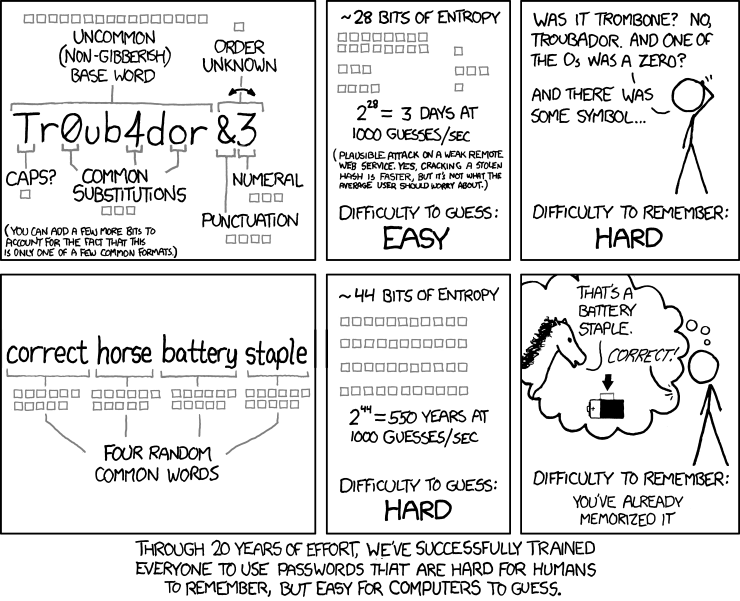
- (Optional) What do you think of the statement the comic makes? Is the password scheme from the comic (four 3-to-8 letter words) safe? What would you recommend to your friends and family, in terms of password management? -->
Counting
One of the first things you learn as a child is how to count. Questions about "how many" are fundamental to how mathematicians think about numbers.
In these lessons, we'll focus on counting elements of sets, in different ways. How many possible combinations of toppings are there for your pizza? How many different possibilities exist for the end of season rankings for a sports league? How many distinct passwords are possible, given a set of rules?
Topics
- counting finite sets
- combinations
- permutations
- factorials
- counting infinite sets: cardinality
- binomial theorem
Resources:
- Chapter 1 of Discrete Mathematics: An Open Introduction, 3rd edition
- Chapter 3 of Introductions to probability
- Instructor reading
Guiding Question Week 5
Our class needs to send 3 representatives to a mathematics competition. How many possible teams could represent us in that competition? Without additional research, think through how to compute that number, and share you reasoning.
Permutations
Key Ideas:
- Defining the concept of a permutation.
- Introduce notation and mathematical intuition behind computing permutations.
Definition
A permutation is a potential rearrangement of elements. For example, the alphabet as we know it, from a to z, is one possible way of ordering the 26 letters. The aim of this first section is to develop the mathematical tools to answer questions like "How many other alphabets could there have been?" we will revisit this further down, but let's start with smaller examples.
Say you have three classmates that are running late: Emmanuel, Kwasi, and Maya. You start wondering in what order they will show up - assuming none of them show up at exactly the same time.
- Emmanuel, Kwasi, Maya
- Emmanuel, Maya, Kwasi
- Maya, Kwasi, Emmanuel
- Maya, Emmanuel, Kwasi
- Kwasi, Emmanuel, Maya
- Kwasi, Maya, Emmanel
As far as I can tell those are the possible ways we can see our classmates coming through. six total permutations. Regardless of what the sequence is, if you have a sequence of three elements, there are six permutations to it. How can we shuffle the letters abc? well we have abc, acb, bca, bac, cab, cba. 6 options as well.
Let's simplify even further, and build up our intuition from an even more basic example:
-
A sequence of one elements only has one possible permutation. You can't shuffle a deck that contains only 1 card. So if our elements are only the letter 'a', then 'a' is the only permutation possible.
-
If we have two elements, a and b, how many permutations do we have? you can quickly intuit that there are 2: ab and ba. Let's dissect this a bit further though: Any permutation will have two elements. You can imagine that there are 2 slots available to put letters in. How many options do we have to put in the first slot? we could put either a or b. Once we've done so, how many options do we have for the last slot? just one, the letter we did not chose at the beginning.
-
With three elements now, a and b and c. There are now three available slots. How many options do we have to put in as the first letter of our permutation? 3. At that point, we are left with 2 slots to fill, and 2 letters to insert them in. This is the same as the problem above, so we know there are two options to complete the permutation. So given that there are 3 options for the first slot, then 2 to continue, we get the total of six permutations.
Let's do it one more time! a, b, c, d. There are four options for the first letter, and we are left to organize three letters in three slots, which we've already established to be six permutations. This gives us a total of 24 options.
Notation:
First, let's define the factorial notation. $ n! = n . (n-1) . (n-2 )...1 $. In plain english, we read that n factorial is the product of n, n-1, n-2, etc. all the way up to 1.
We can therefore define the number of permuations of n distinct elements as n!
So to go back to our original question: How many potential orders could there have been? well there are 26 letters, so let's compute 26!. This should equate to approximately 403 million billion billion - yes, there are no typos here - different possible permutations. As you can see, with as simple a set as the 26 letters, we would quickly have to perform a tremendous amount of computation and store a lot of data if we wanted to keep a record of every possible permutation of the alphabet.
Special case: Zero!
What shoud 0! be equal to? this is a tricky one to define, but we can reach a definition from the following observation.
Notice that $ \frac{n!}{n} = \frac{n . (n-1) . (n-2 )...1}{n} $
As we cancel out n from both parts of the fraction, we obtain $ (n-1) . (n-2 )...1 = (n-1)! $ by definition
Applying this to n = 1 we obtain:
$ \frac{1!}{1} = (1-1)! $
$ \frac{1}{1} = 0! $
Thus we define 0! to be equal to 1 moving forward!
Permutations Video
k-permutations:
Sometimes, we do not care about the entire set of elements, but rather just a subset of it. For example, there are 32 teams joining the world cup. How many permutations are there for the top three? By our current logic, this means we have three slots to fill. How many teams could take the first slot and win the world cup? well there are 32 options. In the next slot, we are left with 31 options, and finally, 30 options, so 32.31.30 gives us 29760 possible permutations to get to the top three!
This can be generalized in the following notation. We call a k-permutation of n elements the number of ways to arrange k elements from a set of n distinct ones. The number of these permutations can be computed as follows:
$$P(n, k) = \frac{n!}{n-k!}$$
More simply, we want the first k terms of the factorial computation, not all of them. We can obtain that mathematically by divinding n! by (n-k)!, leaving us with k elements.
k-permutations Video
References:
For further details, you can read through the following chapters:
Permutations with repetition
Key Ideas:
- Highlight the difference between permutations with replacement, and premutations with limited repeated elements.
- Introduce notation and mathematical intuition behind computing permutations with forms of repetition.
Repetitions:
Both the formulas we have shown so far for permutations fundamentally rely on the set of elements being unique, but what if there is some repetition? There are two types of problems that will force us to change our approach.
Repeated elements:
For this first category of problems, we have elements in our sequence that are equivalent to each other. let's look at an example. If our sequence of elements are a, a, and b, the possible permutations are:
- aab
- aba
- baa
We only find three permutations this time, instead of the six when we had all distinct elements. How do we find a pattern we can generalize here? Let's label our two a's. Now our sequence is $a_1, a_2, b$. When we look at the permutation aab, we could've picked either a for the first two slots. So we could've picked $a_1a_2b$ or $a_2a_1b$ and the result would've been the same.
In other words. When we have two slots dedicated to the letter a, we can distribute $a_1$ and $a_2$ across them. How many ways can we do that? it would be 2 factorial!
So, for each of our original permutations, there is one other one that is equivalent to it, as it's simply a permutation of the different a's, which is why we end up ulitmately with $\frac{6}{2} = 3$ different permutations
More generally we can say that if we have n elements such that $n_1$ of them are of type 1, $n_2$ elements of type 2, all the way up to $n_k$ elements of type k, then we can compute the number of permutations of all those elements as $\frac{n!}{n_1!n_2!...n_k!}$
Time for an example: How about if we had two a and two b as our elements, how many permutations are there? we know we have 2 elements of the same type a, then another two elements of the same type b. Our number of permutations should then be: $\frac{4!}{2!2!} = \frac{24}{4} = 6$
Let's try to list them out:
- aabb
- abab
- abba
- bbaa
- baba
- baab
Replacement:
Our second style of problems is known as replacement problems. In these kind of problems, putting an element from our sequence in a given slot does not prevent it from being added to another slot in our permutation. Imagine for example that while you step away from your laptop, a cat walks accross your keyboard. It presses the keyboard 4 times, then runs away as you come back.
Assuming for a moment that each letter on your keyboard is equally likely to be pressed - how many possible words could the cat have typed while you were away? Let's think about it.
Our sequence of elements here are all the 26 letters of the alphabet. We are looking for how many 4-permutation can be generated, but allowing for the fact that the cat can press the same key many times.
So how many options do we have for the first slot? 26, as with our previous examples. How about the second slot? well all the letters are still fair options - typing 'a' the first time does not prevent us from typing 'a' again, so it's 26 options once again.
The same logic applies for the third and fourth slot. This leaves us with $26 . 26 . 26 . 26 = 26^{4} $ possible permutations.
Generally speaking then, a k-permutation of a sequence of n elements that allows replacement can be computed as $k^n$
References:
For further details, you can read through the following chapters:
Combinations
Key Ideas:
- Defining the notation and formula for combinations
- Highlighting the binomial coefficient visually
Definition
Picture this: It's a hot day, and you stumble into a juice vendor. They have 5 different fruits: Bananas, Oranges, Guava, Strawberries, and Pineapple. You can combine any three fruits into a juice. How many possible juices are there?
We may be tempted to immediately apply permutations here, and compute $P(5, 3) = \frac{5!}{2!} = 60$ different options. This is a good start, but a key observation here is about order
When dealing with permutations, the order of each element is highly relevant. It's inherent in the formula that picking Bananas then Oranges then Guava is different from picking Oranges then Guava then Bananas.
However, I'd argue that once we blend them all into juice, the order in which we put them in does not matter all that much!
So how do we find a more accurate approach? Let's think about it in similar fashion as with permutations with repetition: There are a lot of permutations that are effectively the same. If I pick Bananas then Oranges then Guava, no matter how many times I rearrange those fruits, as long as the exact same three are present we obtain the same juice.
How many ways are there to rearrange three elements? 3 factorial!
So our total number of possible juices needs to be further divided by 3! = 6, giving us 10 different options. We can list them intuitively:
- Bananas, Oranges, Guava
- Bananas, Oranges, Strawberries
- Bananas, Oranges, Pineapple
- Bananas, Guava, Strawberry
- Bananas, Guava, Pineapple
- Bananas, Strawberry, Pineapple
- Oranges, Guava, Strawberries
- Oranges, Guava, Pineapple
- Oranges, Strawberries, Pineapple
- Guava, Strawberries, Pineapple
Which gives us 10 different combinations. Let's formalize our formula and notation.
Notation
The number of ways we can pick k elements out of n different choices is denoted by the symbol $\binom{n}{k} = \frac{n!}{k!(n-k)!} $. We read this as n choose k. More formally, this is also refered to as the binomial coefficient
This formula has some interesting properties: What is $\binom{n}{n}$? How many ways are there to choose n elements from a set of n? there should only be one way, which works out once we plug the values in: $\frac{n!}{n!(n-n)!} = \frac{n!}{n! . 1} = 1$
How about $\binom{n}{0}$? well plugging into our formula we get $\frac{n!}{0! (n-0)!} = \frac{n!}{n! . 1} = 1$. This is odd once you word it out in english, but still makes sense: How many ways can you choose 0 elements from a set? well only one way: Don't choose anything. Interestingly though, we notice that $\binom{n}{0}$ = $\binom{n}{n}$ = 1
This symmetric pattern continues. Let's look at two other scenarios:
$\binom{n}{1} = \frac{n!}{1!(n-1)!} = \frac{n!}{(n-1)!} = n$
Once again this makes sense in plain english: How many ways are there to pick one element from a set of n? n different ways - you could pick any of the elements
How about $\binom{n}{n-1}$? Well: $\binom{n}{n-1} = \frac{n!}{(n-1)!(n-(n-1))!} = \frac{n!}{(n-1)!} = n$
Interestingly, we obtain the same result! $\binom{n}{1}$ = $\binom{n}{n-1}$ = n. We can make sense of this logically: Choosing n-1 elements from a set of n is effectively the same as picking 1 element not to choose.
This symmetric pattern continues, as $\binom{n}{k}$ = $\binom{n}{n-k}$ for all integers $0 \le k \le n$. This pattern is further explored in the diagram below

Notice the pattern: Starting from the top, the left and right edges of the triangle consist of the number 1
Every other spot is the sum of the two numbers above it. How does this connect to combinations? you can view the topmost row as mapping out to $\binom{0}{0}$, which equals 1
The second row, from left to right, represents $\binom{1}{0}$ and $\binom{1}{1}$ The third one, once again from left to right, represents $\binom{2}{0}$, $\binom{2}{1}$, and $\binom{2}{2}$
This makes pascal's triangle a handy tool if you are working on combination problems.
References:
For further details, you can read through the following chapters:
Binomial Coefficients
Key Ideas:
- Introducing visual methods for solving combinations with repetition
- Determining formulas for combinations with repetition
Combinations with repetitions
The clasical example for combinations with repetitions is delicious: Ice cream flavours. Say an ice cream shop offers Vanilla, Chocolate, and Caramel Ice cream. You can get two scoops with your flavors of choice. Nothing stops you from going double Chocolate! This is an instance where choosing a given element does not prevent you from selecting it again.
How can we compute this effectively? To build up intuition for this, I recommend you watch this video first
Once you have watched it, it should be clear why selecting k elements from a set of n while allowing repetition is computed as $\binom{n + k - 1}{k}$. Going back to our icecream example then, picking 2 flavors with repetition from a selection of 3 gives us $\binom{4}{2}$
Applications
Beyond problems where it is explicit that you can make choices with repeated elements, this approach can be used creatively in problems that don't seem to be about combinations in the first place.
Take a look at the following equation. Assuming $x, y, z \in \mathbb N$, let x + y + z = 7. How many solutions are there to this equation?
One way to tackle this is to turn it into a combination problem: The above equation is equivalent to x + y + z = 1 + 1 + 1 + 1 + 1 + 1 + 1. Each of our three variables will contribute some amount of 1's to the sum total.
Therefore, we can think of this as having to choose which 1's belong to x, which 1's belong to y, and which 1's belong to z. In this case. our set is {x, y, z}, and we will be making 7 choices from that set.
Applying our formula, this gives us $\binom{7+3-1}{7} = \binom{9}{7} = 36$ different solutions.
With this, we are now ready to transition to probability - the most direct application of all our counting strategies.
Practice Problems Week 5
- You may collaborate and are encouraged to collaborate with your peers. If you do, be sure to understand the material and write it out in your own words.
There is no requirement to submit the material, but this will help you solidify the concepts.
Instructions:
-
The door to a building has a lock which has 5 buttons numbered from 1 to 5. The combinations of numbers that opens the lock is a sequence of 5 numbers and is reset every week.
a. How many combinations are possible if every button must be used once?
b. Assume that the lock can also have combinations that require you to push 2 buttons simultaneously, and then the other three one at a time. How many combinations does this permit? To clarify, in a sequence of 5 buttons, 2 consecutive buttons must be pressed at the same time to be considered correct.
-
A computer has 3 processors that receive n tasks. Tasks are assigned to the processors purely at random, meaning that all $3^n$ possible assignments are equally likely. How many possible assignments are there where exactly one processor has no task assigned?
-
In how many ways can we choose five people from a group of ten to form a basketball team?
-
Show that $\binom{n}{k} = \binom{n-1}{k-1} + \binom{n-1}{k}$
-
Someone wants to color their fingernails on one hand using at most 2 of the colors red, yellow, and blue. How many ways can they do this?
References:
These problems were drawn from chapter 3 of Introductions to probability as well as Discrete Mathematics- An open introduction
Assignment 5
Complete the assignment on Gradescope using the link below.
After you have completed the assignment, export a PDF of the completed assignment and upload to Anchor below.
Probability
I've chosen a secret number between 1 and 100.
How likely is it that you can guess the number in one try? What about ten tries? What if you knew that I was more likely to pick an odd number?
Probability is about the chances that an event happens. These lessons will focus on the rules you can use to prove statements about events that aren't certain.
Topics
- Definitions: events, randomness and uncertainty
- Probability spaces, sets, and distributions
- Conditional probability
Course Intro Video
Resources:
Guiding Question Week 6
Some probabilities are pretty easy to deduce intuitively. How likely is it that when you flip a coin, it lands on tails? Over the course of next week, we will practice techniques to make it simple for us to compute more complex probabilities. Let's warm up with a question about celebration!
- How likely do you think it is that you share a birthday with one of your classmates?
- How likely do you think it is that two of your classmates share a birthday with each other?
If you are comfortable with it, this would be a great opportunity to share your birthday on a class calendar so we can confirm if our math makes sense. Who knows, we might just figure out that we will have a large party in a few weeks!
Probability
Key ideas
Intro & Definitions
We talk of odds and chances very often, but rarely in a mathematically sound way! It has become a recent meme of late that any outcome is a 50/50: It either happens or it doesn't.
As motivating as that statement is, it is far from mathematically accurate. We will get into the fundamentals of probability theory over the next week. As a topic, probability will have us apply our understandings of Sets, Permutations & Combinations, as well as some proofs. If you feel shaky on any of those topics, make sure take some time to review them, and come through to office hours for support.
Without further ado, let's define some key terms for probability:
- Experiements: When an experiment occurs, we obtain one specific outcome
- Sample Space: The sample space of an experiment is the set of all possible outcomes of that experiment
- Event: This is a subset of the sample space
Example 1: coin toss
Let's quickly clarify the terms with the simplest experiment I can think of: Flipping a coin.
- Flipping the coin is the experiment. The outcome of which will be that we see either heads or tails.
- Therefore, our sample space is $S = \{H, T\}$
- We can describe an event $E = \{H\}$ to represent that we get heads when we flip our coin.
How does this translate to probabilities? Fundamentally, the Probability of a given event $E$ occuring is equal to $\frac{|E|}{|S|}$
In simpler english, we are looking at the ration of "outcomes that make up the event" to "how many possible outcomes are there" In this case. The probabilit of $E$ is represented as $P(E) = \frac{|E|}{|S|} = \frac{1}{2}$ as expected.
Example 2: rolling dice
Let's look at another example: Rolling a six-sided dice. Our sample space is $S = \{1, 2, 3, 4, 5, 6\}$
How likely are we to roll an odd number? you'll probably immediately know that it is 50%, but let's apply the new vocabulary we are learning.
Let $E_{odd}\ = {1, 3, 5}$ represent the event that roll an odd number.
Therefore, $P(E_{odd}) = \frac{|E_{odd}|}{|S|} = \frac{3}{6} = \frac{1}{2}$ as expected.
Example 3: The lottery!
While it may be helpful to explicitly define the sample space and the subset that makes up a given event. That is not always feasible though, but all we need is figuring out
Imagine we run a lottery. We will randomly create a sequence of 5 distinct numbers between 0 and 9, the winning combination. Participants can submit their own sequence of 5 numbers, and win the big prize if they match the sequence we picked. What is the probability that you win this lottery?
Let $E_{win}$ represent he event that we win the lottery. There is only one winning combination, so $|E_{win}| = 1$. That's the first information we need to get our answer.
Now what about our sample space? Last week has luckily given us the tools needed to compute how many such sequences we can have: We are trying to find how many 5-permutations there are of the 10 numbers we can use. The formula for this is $P(10, 5) = \frac{10!}{10-5!} = 10.9.8.7.6 = 30240$
This allows us to compute that our probability of winning $P(E_{win}) = \frac{1}{30240}$. Not particularly enticing! How about we offer participants a chance to win a lesser price.
We're willing to give a second prize to anyone who guesses the same numbers, but in a different order. Our sample space remains unchanged, but how many outcomes fit our new event, $E_{secondPrize}$? Think about it for a few minutes before proceeding.
This is a permutation problem. Given a sequence of 5 distinct digits, how many ways do we have to shuffle them? recall from last week that there are 5! different ways to organize 5 elements. So is that representative of $|E_{secondPrize}|$? not quite!
One of these permutations represents the winning sequence! if we pick that one, we'd win the first prize, not the second. Therefore, $|E_{secondPrize}| = 5! - 1$
This gives us that $P(E_{secondPrize}) = \frac{119}{30240}$ Still not great odds, but 119 times more likely than winning.
Key theorems:
In this section, we formalize some theorems regarding probability. These will form the basis for you to be able to prove more complex statements regarding probabilities.
Consider an experiment with sample space $S$
Theorem 1:
$P(E) \ge 0 \forall E \subset S$.
Probabilities can never be negative by definition, as the cardinality of a set is always greater than or equal to 0.
Theorem 2:
$P(S) = 1$.
This is trivially shown from the formula for computing probabilities, as $\frac{|S|}{|S|} = 1$. In other words. The probability of any of the possible outcomes happening is 1. This also makes up the upper bound of what the probability of any event can be.
Theorem 3:
if $E \subset F \subset S$, then $P(E) \le P(F) $.
This follows from the fact that given that E is a subset of F, $|E| \le |F|$
In the next section, we will look at computing the probabilities of multiple events at the same time, connected by a logical connector.
Probability Spaces Video
References
Chapters 1.1 and 1.2 of Introductions to probability
Combining events
Key ideas
And
What is the probability of satifying two different events at once? Let's consider a game that involves rolling two dice at the same time.
In this case, our sample space S has 36 different outcomes, which we can visualize in the table below. The top row represents the value of the first dice, the leftmost column the values of the second. The pairs inside the table show all our possible outcomes:
| 1 | 2 | 3 | 4 | 5 | 6 | |
|---|---|---|---|---|---|---|
| 1 | (1,1) | (1,2) | (1,3) | (1,4) | (1,5) | (1,6) |
| 2 | (2,1) | (2,2) | (2,3) | (2,4) | (2,5) | (2,6) |
| 3 | (3,1) | (3,2) | (3,3) | (3,4) | (3,5) | (3,6) |
| 4 | (4,1) | (4,2) | (4,3) | (4,4) | (4,5) | (4,6) |
| 5 | (5,1) | (5,2) | (5,3) | (5,4) | (5,5) | (5,6) |
| 6 | (6,1) | (6,2) | (6,3) | (6,4) | (6,5) | (6,6) |
Let's consider $E_1$ to represent the event that you roll at least a single 1. You can see that there are 11 scenarios that make up this event. They are shown in bold in the table below:
| 1 | 2 | 3 | 4 | 5 | 6 | |
|---|---|---|---|---|---|---|
| 1 | (1,1) | (1,2) | (1,3) | (1,4) | (1,5) | (1,6) |
| 2 | (2,1) | (2,2) | (2,3) | (2,4) | (2,5) | (2,6) |
| 3 | (3,1) | (3,2) | (3,3) | (3,4) | (3,5) | (3,6) |
| 4 | (4,1) | (4,2) | (4,3) | (4,4) | (4,5) | (4,6) |
| 5 | (5,1) | (5,2) | (5,3) | (5,4) | (5,5) | (5,6) |
| 6 | (6,1) | (6,2) | (6,3) | (6,4) | (6,5) | (6,6) |
Similarly, $E_6$ represents the event that you roll at least a single 6. The table below highlights the 11 outcomes that make up that scenario as well.
| 1 | 2 | 3 | 4 | 5 | 6 | |
|---|---|---|---|---|---|---|
| 1 | (1,1) | (1,2) | (1,3) | (1,4) | (1,5) | (1,6) |
| 2 | (2,1) | (2,2) | (2,3) | (2,4) | (2,5) | (2,6) |
| 3 | (3,1) | (3,2) | (3,3) | (3,4) | (3,5) | (3,6) |
| 4 | (4,1) | (4,2) | (4,3) | (4,4) | (4,5) | (4,6) |
| 5 | (5,1) | (5,2) | (5,3) | (5,4) | (5,5) | (5,6) |
| 6 | (6,1) | (6,2) | (6,3) | (6,4) | (6,5) | (6,6) |
What is the probability that we achieve both $E_1$ and $E_6$? In plain english this is the probability that we roll at least one 1 and one 6.
This can be constructed as a brand new event $G$ which consists of the outcomes that belong to both $E_1$ and $E_6$, or more directly, $G = (E_1 \cap E_6)$.
We therefore can compute $P(G) = P(E_1 \cap E_6) = \frac {|E_1 \cap E_6|}{|S|}$. From the table, you can see that only (1,6) and (6, 1) belong to both evets. This gives us $\frac {2}{36}$
How about the following scenario:
Let $F = \{(6,5), (5,6), (6,6)\}$ represent the event that the sum of your dice rolls is greater than 10. What is the probability that both $E_1$ and $F$ occur? as we've shown, $P(E \cap F)$ is equal to $\frac {|E \cap F|}{|S|} = \frac {0}{36}$
Disjoint sets:
A quick aside before we proceed: We consider two sets A and B to be disjoint if $A \cap B = \emptyset$. In other words, two disjoint sets have no elements in common.
Broadening the definition, we say that two events are disjoint if they share no outcome in common. This means that the probability of two disjoint events occuring at the same time is always 0, as they have no intersection.
Or
How about the probability that we satisfy either of two events? Let's start with the same example we left off with, where:
- $E_1$ represents the event that you roll at least a single 1.
- $F$ represent the event that the sum of your dice rolls is greater than 10.
We can create a new event $G$ which consists of the outcomes that belong to either $E_1$ or $F$, or more directly, $G = E_1 \cup F$. It follows then that $P(G) = P(E_1 \cup F) = \frac {|E_1 \cup F|}{|S|}$
How do we compute $|E_1 \cup F|$? luckily, we know by definition of these two events that they are disjoint, so $|E_1 \cup F| = |E_1| + |F|$.
This means that $P(E_1 \cup F) = \frac {14}{36}$
This leads us to our fourth key theorem:
Theorem 4:
If A and B are disjoint events with sample space S, then $P(A \cup B) = P(A) + P(B)$
We can prove this directly: $P(A \cup B) = \frac{|A \cup B|}{|S|}$ Given that the two sets are disjoint, we have $|A \cup B| = |A| + |B|$
Therefore, $P(A \cup B) = \frac{|A| + |B|}{|S|}$
$P(A \cup B) = \frac{|A|}{|S|} + \frac{|B|}{|S|}$
$P(A \cup B) = P(A) + P(B)$
How about non-disjoint events?
Before talking about events, let's focus on sets: We can quickly see visually that if two sets A and B have some elements in common, we can't simply say that $|A \cup B| = |A| + |B|$ The elements in common would be getting counted twice! Therefore, the correct approach here is $|A \cup B| = |A| + |B| - |A \cap B|$ so that we cancel out the elements that show up in both sets.
This same logic applies to figuring out the probabilites of non-disjoint events. Let's go back to our previous examples:
- $E_1$ represents the event that you roll at least a single 1.
- $E_6$ represents the event that you roll at least a single 6.
These events are not disjoint, we know we could achieve both outcomes.
The probability that we roll at least a single 1 or a single 6 therefore is $P(E_1 \cup E_6) = \frac {|E_1 \cup E_6|}{|S|} = \frac {|E_1| + |E_6| - |E_! \cap E_6|}{36} = \frac {20}{36}$
By the same approach of theorem 4, we can generalize the formula for $P(A \cup B) = P(A) + P(B) - P(A \cap B)$
Complements of events
For some sample space $S$, we define the complement of an event $E$ to be all the outcomes that are not present in $E$. Similarly as in sets, we represent the complement of $E$ as $\bar E$.
It follows then that $(E \cup \bar E) = S$
Note that $E$ and $\bar E$ are by definition disjoint, as they will never share outcomes in common.
This means that $P(E \cup \bar E) = P(E) + P(\bar E)$ from Theorem 4
We also know that $P(E \cup \bar E) = P(S) = 1$ from Theorem 2
This enables us to come up with a new, very useful theorem:
Theorem 5
For some sample space $S$ and event $E$: $P(E) = 1 - P(\bar E)$
This is very handy in scenarios where computing $P(\bar E)$ is simpler than computing $P(E)$.
For example, let $E$ be the event that when rolling two dice, you get two different numbers?
By definition, this is 1 minus the probability of obtaining a doubled number. Intuitively, it is simpler to see that there are exactly 6 outcomes where we have doubled numbers: (1,1), (2,2), (3,3), (4,4), (5,5), and (6,6)
Therefore, our probability $P(E) = 1-P(\bar E) = 1 - \frac{6}{36} = \frac {5}{6}$
In the next section, we will get into a different way to connect events together
Combining Events Video
References
Chapters 1.1 and 1.2 of Introductions to probability
Conditional Probability
Key ideas
- Introduce the concept of dependents and independent events
- Define the formula for conditional probability and how it is affected by independent events
Do these events matter?
Picture this. Your team has been competing with a rival school for many years now, and you have been keeping track diligently of your wins and losses. Your team's record so far is that you have won 70 games and lost 50. With this in mind, you are confident to head into the next game.
One of your older classmates however is not as confident, and she says that "Mr.O will be the referee this time around, he doesn't like us". This leaves you exceedingly curious. Time to go back to your data and see if the referee really influences your chances to win:
| Referee | # of wins | # of losses | Total |
|---|---|---|---|
| Mr C. | 20 | 8 | 28 |
| Mr O. | 6 | 12 | 18 |
| Mr S. | 44 | 20 | 64 |
| Total | 70 | 50 | 120 |
Our overwall probabilities to win are quite clear: $P(Winning) = \frac{70}{120}$, or approximately 0.58. The question is: Is our chance of winning independent on who is the referee? or does our chance of winning depend on who will be the referee for the game?
Let's pause for a second to start some definition. We can represent the probability that an event $E$ occurs given an event $F$ by the notation $P(E|F)$
We say then that two events $E$ and $F$ are independent if $ P(E) = P(E|F)$. In other words, whether or not the event $F$ occurs, the probability of $E$ happening is unchanged.
Conversely, if $ P(E) \neq P(E|F)$, then the two events are dependent - $F$ can influence $E$, and vice versa.
Let's go back to our example above. What is P(Winning | Mr.O is the referee)? We do not have a set formula for this yet, but let's think about it. We have played a total of 18 games refereed by Mr.O, and won 6. The chances of us winning based on this data are therefore P(Winning | Mr.O is the referee) = $\frac{6}{18} = \frac{1}{3} $, noticeably lower than our overall 58% winrate!
This suggests that our two events, Winning and having Mr. O as our referee, are depedent!
Let's dip now into the more theoretical aspects of conditional probability so that we can establish a general formula for it.
Conditional probability
Start by watching this video on the fundamentals of Conditional probability. This will visually show where the formula comes from, as well as offer several practice problems.
Conditional probability formula
The probability of event $E$ given event $F$ is computed as $ P(E|F) = \frac{P(E \cap F)}{P(F)}$, given that $P(F) \neq 0$
Independence test
If $A$ and $B$, with $P(A) \neq 0$ and $P(B) \neq 0$, are independent then the following statements are equivalent:
- $P(A) = P(A|B)$
- $P(B) = P(B|A)$
- $P(A)P(B) = P(A \cap B)$
We can reach the second statement from the first as follows:
$P(A) = \frac{P(A \cap B)}{P(B)}$ by definition of conditional probability
$P(B) = \frac{P(A \cap B)}{P(A)}$ given that both $P(A)$ and $P(B)$ are non-zero
$P(B) = P(B|A)$ by definition of conditional probability
And similarly, we can reach the third statement from the first:
$P(A) = \frac{P(A \cap B)}{P(B)}$ by definition of conditional probability
$P(A)P(B) = P(A \cap B)$
The reason we take time to explicitly show that these three statements are equivalent is to offer you flexibility in how to approach problems involving checking for independence and computing conditional probability
Independence and complements
If $A$ and $B$ are independent events, it follows that $A$ and $\bar B$ are independent as well.
Intuitively this should make sense: If $A$ occuring does not influence $B$, then it shouldn't influence $\bar B$. If $P(B)$ doesn't change given $A$ then neither should $1-P(B)$
We can prove this statement directly:
$P(A)P(B) = P(A \cap B)$ by definition of independence
$P(A)(1-P(\bar B)) = P(A \cap B)$ by definition of complement
$P(A) - P(A)P(\bar B) = P(A \cap B)$
$P(A) - P(A \cap B) = P(A)P(\bar B)$
How can we evaluate $P(A) - P(A \cap B)$? This expression represents the probability of event $A$ occuring, minus the probability of event $A$ and $B$ occuring. From a set perspective, this means we care only about the outcomes that belong to $A$ but do not belong to $B$. This can be expressed as $P(A \cap \bar B)$.
Therefore, $P(A)P(\bar B) = P(A \cap \bar B)$
And thus, we have shown that $A$ and $\bar B$ are independent.
Symmetrically, we can use the same approach to show that $ \bar A$ and $B$ are independent, as well as $\bar A$ and $\bar B$
In the next section, we bring all our knowledge together in a case study, and see how we can use code to help us hone our intuition with probabilities.
References:
Chapter 4 of Introductions to probability
A case study: The monty hall problem
Key ideas
- Apply conditional probability in a practical scenario.
- Introduce the ability to run trials in code to build up intuition of probability.
A tricky game show:
Let's consider one of Mathematics' most famous questions: The Monty Hall problem. This problem became famous when it was shared in a journal in 1990:
Suppose you're on a game show, and you're given the choice of three doors: Behind one door is a car; behind the others, goats. You pick a door, say No. 1, and the host, who knows what's behind the doors, opens another door, say No. 3, which has a goat. He then says to you, "Do you want to pick door No. 2?" Is it to your advantage to switch your choice?
Think about it for a moment. What move maximizes your chance of winning: Staying with your first choice? shifting? or does it even matter? Take some time to think through it, and try applying conditional probabilities to figure it out before moving forward.
To clarify the rules of the game:
- You pick a random door out of 3 options.
- The host will then open a door with a goat behind it, and offer you an opportunity to switch.
- The host will never open your door, or the door with the car.
- If the host has options for what door to open, they will pick randomly.
We can define a few events for this: Let $C_1, C_2, C_3$ represent the events that the car is behind door 1, 2, and 3 respectively.
Similarly, let $H_1, H_2, H_3$ represent the events that the host opens door 1, 2, and 3 respectively.
We set a scenario where you initially pick door 1, then the host opens door 2. At this point in time, what is $P(C_3|H_2)$? Are they better than your odds if you stick to your initial choice?
$P(C_3|H_2) = \frac{P(C_3 \cap H_2)}{P(H_2)}$
Let's start by computing $P(H_2)$, following the assumption that you choose door 1.
- If the car is indeed behind door 1, then the host has a $\frac{1}{2}$ chance to open door 2, and a $\frac{1}{2}$ chance to open door 3, as they pick randomly.
- If the car is behind door 2, then the host will open door 3. There is no chance the host opens door 2 in this scenario.
- If the car is behind door 3, then the host will always open door 2.
The car has a $\frac{1}{3}$ chance to be behind any door. This means that the probability the host opens door 2 is $\frac{1}{3} . \frac{1}{2} + \frac{1}{3} . 0 + \frac{1}{3} . 1 = \frac{1}{2}$
Now what is $P(C_3 \cap H_2)$? As mentioned, if the car is behind door 3 then the host is guaranteed to open door 2, so this is the same as the odds that the car is behind door 3. $P(C_3 \cap H_2) = P(C_3) = \frac{1}{3}$
Plugging this in, we get that our conditional probability $P(C_3|H_2) = \frac{2}{3}$. We have a 66.67% chance to win by switching instead of sticking to our initial guess!
This is a surprising result to many - in fact, thousands of readers sent very angry letters when the solution was published. The reasoning is sound though.
In general, conditional probabilities push us to be very accurate about the situations we are in and question some of our biases about what events are indeed connected or not.
Running trials
As an aside - as developers, you can always easily confirm your computations and intuitions for probability in code. The linked python script defines two functions:
- The first function simulates the scenario where we always stick to our first choice. This function returns true or false if our guess turned out correct.
- The second function simulates the scenario where we always switch our choice after the host opens a door. It also returns true or false if the guess turned out correct.
We run both those functions 500 times, and track how often each returns True. The results confirm what we computed earlier: The odds of winning when sticking to our choice are about 33%, whereas the odds of winning when changing doors are 66%.
Two things to note before we wrap up this week:
-
As unlikely as it is, it is possible for our first strategy to guess correctly for all 500 attempts. Our code would then report a 100% success rate. Never run trials like this only once, or on small samples.
-
As you grow more confident with Python, you will be able to simulate increasingly more complex situations. However, it is your understanding of the underlying statistics that will allow you to write the correct code to make it happen. There is no silver bullet here! it's up to you to bring your knowledge into the code.
Practice Problems Week 6
- You may collaborate and are encouraged to collaborate with your peers. If you do, be sure to understand the material and write it out in your own words.
There is no requirement to submit the material, but this will help you solidify the concepts.
Problems
-
We flip a coin three times. The set of all possible outcomes is: $\omega = \{HHH, HHT, HTH, HTT, TTT, TTH, THH, THT\} $
Each of the following events are subsets of $\omega$. For each event, describe the event in english, then compute the probability of it occuring:
- $E_1 = \{HHH, TTT\}$
- $E_2 = \{HHT, THH, HTH\}$
- $E_3 = \{HHH, HHT, HTH, HTT\}$
-
If A, B, and C are three events, show the following:
$P( A \cup B \cup C) = P(A) + P(B) + P(C) - P(A \cap B) - P(B \cap C) - P(A \cap C) + P(A \cap B \cap C)$
Hint: You might start by showing the result for just events A and B. It may also help to draw a Venn diagram.
-
From a deck of five cards numbered 2, 4, 6, 8, and 10, respectively, a card is drawn at random, then placed back in the deck. This is done three times, and you are told that the sum of the numbers on the three draws is 12. What is the probability that the card numbered 2 was drawn exactly two times, given that the sum was 12?
-
One coin in a collection of 65 coins has two heads. The rest are fair. If a coin, chosen at random from the collection and then tossed, turns up heads 6 times in a row, what is the probability that it is the two-headed coin?
-
You are given two urns and forty balls. Half of the balls are white and half are black. You are asked to distribute the balls between the two urns with no restriction on the number of white or blank in an urn. An urn will be chosen at random, and a ball will be drawn from it at random.
How should you distribute the balls in the urns to maximize the probability of drawing a white ball? Justify your answer.
Extension (optional): Prove your answer.
One approach might be to write a Python program that loops through every possible arrangement, calculates the probability of drawing a white ball for each arrangement, and finds the maximum probability.
References:
These problems were drawn from chapters 1.2 and 4.1 of Introductions to probability
Assignment 6
Complete the assignment on Gradescope using the link below.
After you have completed the assignment, export a PDF of the completed assignment and upload to Anchor below.
Review and Preview
This week will be a review of what you've learned so far, and a preview of how it connects to other branches of computer science and mathematics.
There won't be a regular problem set or weekly question this week. Instead, you'll spend time finishing up any previous work, reflecting on what you've learned, and looking ahead to other topics.
Future Topics
Limits
Limits are a fundamental tool in the toolbox for proving statements for continuous sets, like the real number line. Limits are also the backbone of Calculus. We care about limits because they help us think about what happens to functions across all cases - not just a few carefully chosen ones. This is particularly important when we're evaluating how fast a program will run, or how much space it will take up, given different inputs.
- Discrete vs continuous
- What is a limit?
- Infinitesimally small: The differential
- Preview of differential and integral calculus
Complexity
Functions and Relations
We can relate numbers to other numbers in tons of different ways. You've been using relations and functions to 'get from' one set of numbers to another for a while: every time you see an expression like x + 7 or sin(y), that's a function. The x and y are the input of the function, and the + 7 or sin() tell you how to get to the output.
In the next few lessons, you'll learn more about the rules of functions and relations, and how we can prove statements about them.
Topics
- definitions: functions, relations, domain, codomain, and range
- function composition
- the 'jections: injection, surjection, bijection (one-to-one, onto, and invertible)
- pigeonhole principle
Resources:
- Sections B2 & B3 from Introduction to Algorithms, Third edition.
- Discrete Mathematics: An open textbook section 0.4
Guiding Question Week 8
We have been able to solve so many day-to-day problems using computers. Many of these problems fundamentally are about transformation: Taking some input, and turning it into some new, more useful output.
Take a look at the following three links: https://www.unitconverters.net, https://image.online-convert.com/convert-to-jpg, and https://convertio.co/ocr.
Take some time and test each of these tools.
- For each of the tools linked, what kind of input do they expect to receive? what kind of output do they produce?
- Make a guess as to how each one of them could be working.
- Based on that guess, do you think it's possible to go the other way around? In other words, use the output to produce the input, somehow?
Relations
Key Ideas:
- Define relations as substes of a cartesian product
- Introduce the concept of equivalence relations
Relations
Relations are a cornerstone of mathematical thinking, and arguable of thinking in general. They refer to a mapping of elements, inputs and outputs. If you've used some kind of a table before, then you are using a relation. For example if we wanted to track how much money friends contributed to some fundraisers, we could organize this in a table as follows:
| Name | Contribution |
|---|---|
| Ife | 200 |
| Tolu | 150 |
| Olivia | 150 |
| Tolu | 100 |
We could map out data about students' attendance in a school, for example:
| Name | Missed sessions |
|---|---|
| Tomi | 0 |
| Edward | 3 |
| Kwasi | 1 |
| Afia | 1 |
A relation connects elements from a specific set - for example, a series of names in the above tables - and maps them onto values from another set.
The relation then is really a set of pairs, where each pair contains an input and its corresponding output. For example we can restructure them as follows:
- Table 1: {(Ife, 200), (Tolu, 150), (Olivia, 150), (Tolu, 100)}
- Table 2: {(Tomi, 0), (Edward, 3), (Kwasi, 1), (Afia, 1)}
Cartesian products
Let's look at table 2. The "inputs" for his relation come from a set of names, let's call it $A = \{Tomi, Edward, Kwasi, Afia\}$.
These names are mapped onto an integer. Let's say that this course has 20 sessions overall, so the most a student can miss is 20, and the least is 0. We can define the set of outputs as $B = \{0, 1, 2, ... 20\}$.
To describe our relations, we create a pair of elements (a, b) such that $a \in A, b \in B$. It would not make sense for this relation to include a value like (Tomi, -3), or (Kwasi, Kwasi).
We have a handy way to describe this idea of pairing elements from two sets: Given two sets A and B we define the cartesian product of these two sets as $A \times B = \{(a, b) \forall a \in A, \forall b \in B\}$. In other words, this is the set of all possible pairs of values coming from both sets.
Note here that these pairs are ordered. (Tomi, 0) is not the same as (0, Tomi). Therefore if A and B are two different sets, then $A \times B \neq B \times A$
What is the cardinality of $A \times B$? We should have all the tools needed to compute that: We have $|A|$ options for the first element of the pair, and $|B|$ options for the second. This gives us that $|A \times B| = |A|.|B|$
Formal definition
We can now give a proper definition of what a relation is: A relation is any subset of a Cartesian product.
Given two elements $a \in A, b \in B$ and relation R which is a subset of $A \times B$, we can write $a R b$ to indicate that the pair $(a,b) \in R$
Equivalence relations
Note that the two sets of inputs and outputs do not need to be different, and we can define relations on a cartesian product $S \times S$, the product of a set S with itself.
This enables us to create relations that capture an interesting property: That some values are equivalent to each other, i.e that we could swap them out for each other without issue.
for example let's consider the cartesian product of the set $\mathbb Z$ with itself. This gives us the set of all pairs of integers.
Consider then the relation $R = \{(x, y) | x^2 = y^2\}$. This relation is a subset of $\mathbb R \times \mathbb R$ that only keeps the pairs of numbers that have the same squared value. We will show how this relation R is an equivalence relation
Is $(3,4) \in R$? no, as we can easily show that $3^2 \neq 4^2$. In other words, 3 is not equivalent to 4 in this relation.
How about $(3,3) \in R$? It is true as $3^2 = 3^2$. It is somewhat obvious, but 3 is equivalent to itself in this relation.
How about $(2,-2) \in R$ That is also true, as $2^2 = (-2)^2$. How about if we flip it? is $(-2,2) \in R$? yes indeed.
More generally, an equivalence relation $R$ on a set $S$ requires 3 properties to be true:
- R is Reflexive: This means that $\forall x \in S: xRx$
- R is symmetric: This means that $\forall x, y \in S: xRy \implies yRx$
- R is transitive: This means that $\forall x, y, z \in S: xRy \land yRz \implies xRz$
Let's go back to $R = \{(x, y) | x^2 = y^2\}$:
- R is reflexive: $\forall x \in \mathbb Z: x^2 = x^2$, so it follows that $(x, x)\in R \forall x \in \mathbb Z$
- R is symmetric: $\forall x, y \in \mathbb Z: x^2 = y^2 \implies y^2 = x^2$ so if $xRy$ then $yRx$ follows.
- R is transitive: if $xRy$ and $yRz$, it follows that $x^2 = y^2 = z^2$ so $xRz$
Do be careful that you need to explicitly cover all three properties to establish an equivalence relation. There are relation that exhibit some but not all of these properties. For example consider the relation $R = \{(x, y) | x \leq y\}$:
- Is R reflexive? yes! we can say that a number is less than or equal to itself
- Is R transitive? yes! if $x \leq y, y \leq z$, it follows that $x \leq z$
- How about the symmetric property? this is where things break! we can say that $(3,4) \in R$ for example, but not that $(5,3) \in R$
We will revisit equivalence relations in a couple weeks as we move into number theory, but for now, let's look into a different type of relations: functions.
Vidro on Relations
References:
chapter 1.2 of Precalculus, 3rd corrected edition by S&Z
Functions
Key Ideas:
- Define the properties of relations that make them functions.
- Introduce notation and definitionsfor functions, domains, codomains, and images.
- Revisit prior content through the lense of functions.
Relations to functions
Every function is a relation, but not every relation is a function. In order to be a function, a relation needs to satisfy one key constraint:
A relation $R \subseteq A \times B$ is a function if and only if $\forall x \in A$, there exists a unique element $y \in B$ such that $xRy$
Let's go back to our previous examples. We had a relation, $Table1: \{(Ife, 200), (Tolu, 150), (Olivia, 150), (Tolu, 100)\}$ to capture donations from people. If I were to ask you how much Ife donated, the answer is clear: 200
But if I were to ask you how much Tolu donated, there is more than one singular answer. Tolu maps to two different outputs. This means there isn't a unique element that the value "Tolu" maps to, so this relation is not a function.
How abot $R_2: \{(Tomi, 0), (Edward, 3), (Kwasi, 1), (Afia, 1)\}$. It is a function indeed, as each name only appears once.
Definition of a function:
We define a function $f: A \to B$ such that all elements of $A$ are uniquely mapped to some element of $B$
- The set $A$ is known as the domain of the function
- The set $B$ is the function's codomain
- We say that $f(x)$ - pronounced "f of x" - is the image of the value x using function f. It follows that $f(x) \in B$
Let's consider two functions, f and g.
we can define $f: \mathbb N \to \mathbb N: f(x) = x^2$ and $g: \mathbb R \to \mathbb R: g(x) = x^2$
Both these functions take an input, then raise it to the power of two. However these are different functions - even though they follow the same logic - as their domains and codomains are different.
This could be clearer if we go back to thinking of sets as relations. The pair (0.1, 0.01) is part of the relation g, but is not part of the relation f
Images of a set:
We can also take images of a set. Let $f: A \to B$ be a function and $C \subset A$
$f(C)$ represents the set of the images of all elements in C, or in other words: $f(C) = \{f(x) \forall x \in C\}$
$f(A)$ represents the set of images of all the elements of our domain. Note that this does not necessarily mean that $f(A) = B$. We can however say that $f(A) \subseteq B$.
Interesting functions and relations:
In this section we cover a few different functions to solidify the concept, revisiting some older topics in the process.
Logical operators:
We can look at many of our logical operators as a function. Let's start with $\lnot$. We can define a function $Not$ as follows:
- The domain is the set $B = \{True, False\}$
- The codomain is also the set $B$
- $not(x) = \lnot x$
Our inputs and outputs in this case are both a single boolean value.
Functions don't necessarily have to take single values as an input. We can define a function $And$ which takes two diffent boolean values.
How can we express all the pairs of boolean values? Let's use the cartesian product:
We can define a function $And: B \times B \to B$:
- The domain of the function is the set $B \times B = {(True, True), (True, False), (False, True), (False, False)}$
- The codomain of the function is the set $B = {True, False}$
- $And(x, y) = x \land y$
Probability distributions:
We can revisit probability as well in terms of functions. Say we want to create a function that gives us the odd that a dice rolls a specific number.
- Our domain is the set $D = \{1, 2, 3, 4, 5, 6\}$
- Our codomain, by definition of probability, is values between 0 and 1. we can define a set $P = \{x \in \mathbb R: 0 \leq x \leq 1\}$. In this case it would also be valid to consider the codomain to be just the element $\frac{1}{6}$, but let's stick with P as our domain.
- Therefore we have our function set up such that $f(1) = f(2) = f(3) = f(4) = f(5) = f(6) = \frac{1}{6}$
This is what we call a uniform probability distribution: All the odds are the same for any of the values. This has been our assumption throughout week 5, but events are not always evenly distributed.
Imagine we have some unfair dice, where a 6 is twice as likely to be rolled than any other number, and all other numbers have the same probability to be rolled as each other. Our domain does not change, neither does our codomain, but our mapping must change!
Well we said that rolling a 6 is twice as likely, so can we define the function like this?
| x | 1 | 2 | 3 | 4 | 5 | 6 |
|---|---|---|---|---|---|---|
| f(x) | $\frac{1}{6}$ | $\frac{1}{6}$ | $\frac{1}{6}$ | $\frac{1}{6}$ | $\frac{1}{6}$ | $\frac{2}{6}$ |
Let's remember that the sum of all our probabilities must add up to 1. Is it the case? Adding all the probabilitis up we get $\frac{7}{6}$ which is greater than 1, so we have an issue.
This is tricky, but we can figure this out. From the definition of this unfair dice, the probability of rolling a one is the same as rolling a two, a three, a four, or a five. The probability of rolling a six is twice as much as rolling one of the other numbers.
So we know that we want $f(1)+f(2)+f(3)+f(4)+f(5)+f(6) = 1$
$5f(1) + f(6) = 1$ since all numbers under 5 have the same probability to be rolled.
$5f(1) + 2f(1) = 1$ since rolling a 6 is twice as likely as rolling a 1.
$f(1) = \frac{1}{7}$
Which gives us our definition:
| x | 1 | 2 | 3 | 4 | 5 | 6 |
|---|---|---|---|---|---|---|
| f(x) | $\frac{1}{7}$ | $\frac{1}{7}$ | $\frac{1}{7}$ | $\frac{1}{7}$ | $\frac{1}{7}$ | $\frac{2}{7}$ |
This kind of function is called a probability distribution, which we will explore a lot more in future classes.
The main takeway to share here is that functions are crafted for a specific purpose. For example, probability distributions have a constraint on them that the sum of all the probabilities must be equal to 1. This allows us to apply our knowledge of statistics, while at the same time looking at it through the lense of functions.
Throughout your studies and careers, you will come up with many functions - often implementing them in code. Be creative! You can set your own constraints and limits to them to solve the problem at hand.
References:
Chapter 0.4 of Discrete Mathematics: An Open Introduction, 3rd edition chapter 1 of Precalculus, 3rd corrected edition by S&Z
Properties of functions:
Key Ideas:
- Introducing Injective, Surjective, and Bijective functions.
- Showcasing techniques for proving whether or not a function shows these properties.
- Introducing the concepts of inverses of a function.
Injective functions
A function is injective if no two elements of the input map to the same element.
Formally, let $f: A \to B$. f is injective if $\forall x, y \in A: f(x) = f(y) \implies x = y$
For example let's consider our $not$ function from the last chapter:
- $not(True) = False$
- $not(False) = True$
So $not$ is injective since we tested all the values from our domain, and none of them shared the same image.
Is the function $And$ injective? We have that $And(True, False) = And(False, False) = False$, so the function is not injective as those two inputs map to the same output.
Visually, we can also express this idea as: There are no two arrows that point to the same element

Showing a functon is injective, or not
To show that a function is not injective only requires a counter example, can you find two distinct elements x and y from the domain such that f(x) = f(y)? if so your proof is done.
Conversely, showing that a function is injective requires showing that $\forall x, y \in Domain: f(x) = f(y) \implies x = y$. This can be done directly in some cases, assuming that you have two values $x, y$ such that (\f(x) = f(y)$, and reaching the conclusion that $x$ and $y$ must be equal.
The contrapositive of our statement above is that $\forall x, y \in Domain: x \neq y \implies f(x) \neq f(y)$, which can make the proof simpler in some cases. You can identify two distinct values $x, y$, and reaching the conclusion that $f(x) \neq f(y)$
Surjective functions
A function is surjective if Every element of the codomain is the image of some element in the domain
Formally, let $f: A \to B$ be a surjective function. f is surjective if that $\forall y \in B, \exists x \in A: f(x) = y$
Going back to our examples, we can quickly see that both the $And$ function and the $Not$ function are surjective as there are outputs that produce True and outputs that produce False.
Let's consider however the function $g: \mathbb R \to \mathbb R: g(x) = x^2$. Is it surjective? consider that $-1 \in \mathbb R$, our codomain. Can we solve the equation $x^2 = -1$?
As we do not have a definition for the square root of a negative number, -1 is not the image of any element from our domain
It follows then that g is not surjective.
Visually, we can also express this property as: Every element in the codomain has at least one arrow pointing to it.

Showing a function is surjective, or not
To show that a function is not surjective requires a counter example: Can you find an element k of the codomain such that $\forall x \in Domain: f(x) \neq k$? This requires some careful thinking for what k is, as well as some insight into the function itself to prove that there is no x in the domain that satisfies f(x) = k
Alternatively, one can also apprach this by looking at the sizes of the domain and codomain: if the codomain is larger than the domain, and each value of the domain maps to exactly one value in the codomain by definition of what a function is, then surely there are elements of the codomain with no source in the domain.
To show a function is surjective requires showing that $\forall y \in Codomain, \exists x \in Domain: f(x) = k$. This is often done in a direct proof. You can define an arbitrary variable $y \in Codomain$, then show that $\exists x \in Domain: f(x) = y$. The crux of this proof often lies in finding an expression of x in terms of y, then establishing that it is indeed a member of the domain.
Bijective functions
Let's think about what it means for a function to be injective: For a given y in the codomain, how many possible values f are there in the domain such that f(x) = y? There can't be two or more, by definition of what it means to be an injective function. There could be none at all, and there could be one. Those are the only options. In other words at most one value in the domain maps to any value in the codomain
Let's consider the same question for surjective functions. For a given y in the codomain, how many possible values f are there in the domain such that f(x) = y? Well there has to be at least one, otherwise we would not be a surjective function.
So what can we say about a function that is both injective and surjective? The most intuitive way to think about it is that for every element of the domain there is exactly one element of the codomain, and vice versa.
Visually, a bijective function looks like this:

Inverting functions
The most powerful property of bijective functions is that they can be inverted. If we have a bijective function $f: A \to B$, we can define it's inverse $f^{-1}: B \to A, f^{-1}(y) = x \iff f(x) = y$
From a visual perspective, this is the function we obtain if we flip all the arrows in the previous image!
The lesson to take here is that a bijective function can be undone. If we have the output of a bijective function, we can reliably reconstruct its original input.
This translates well to functions in a programming context. When defining your own content, it is worthwhile to think about what properties it exhibits. If it is bijective, mapping every possible input to a unique output, then you could write a function that does the opposite of it easily.
If it is not bijective however - say that some of its inputs map to the same output - then it would be quite difficul to reliably undo the action that function performs. If you were provided with that output, how would you decide what input it connects to?
Functions as they are used in programming draw a lot of inspiration from mathematical functions and their properties. Let's explore one final one in the next section.
References:
Chapter 0.4 of Discrete Mathematics: An Open Introduction, 3rd edition chapter 1 of Precalculus, 3rd corrected edition by S&Z
Function composition
Key Ideas:
- Define notation for function composition
- Relate function composition to programming
- Show how established properties of functions translate to compositions
Combining functions
As we think of functions in terms of inputs and outputs, we can imagine a system where the output of a function becomes an input for the next one.
Let's say we have $f: A \to B$ and $g: C \to D$. Could we compose these two functions in a way that the output of the function f becomes an input to function g. For some $a \in A$, we would want to compute g(f(a)). Can we even do that?
It depends. We know that $f(a) \in B$ so as long as $B \subseteq C$, we can apply both functions, one after the other. However, if the codomain of our firt function is not a subset of the domain of the second, this will not reliably be the case. For the rest of these notes we will set things up so that codomains and domains match, but that is something to be cautious of when combining functions on your own.
We can formally define the composition of two functions as a new function. Given $f: X \to Y$ and $g: Y \to Z$ we define the function:
$g \circ f: X \to Z, g \circ f(x) = g(f(x))$.
We use the $\circ$ symbol to denote composition, and we read $g \circ f$ as "g of f"
This translates directly to programming, where you may have seen this syntax before:
	def f(x):
		return x*x

	def g(x):
		return (5*x)-12

	# If we want to compute g of f of x, we can do so like this:
	composition = g(f(1))
	# We first figure out what the value of f(1) is, then we provide that as an input to the g function

	# If this is something you'd want to do often in your code, you could use f and g as building blocks for a new function.
	def g_of_f(x):
		return g(f(x))
You do have to be a bit careful when composing functions together however: We will still be concerned with domains and codomains. Look at this example:
	def f(x):
		return x - 5

	def g(x):
		return 2 / x

	test1 = g(f(10)) # test1 will equal 0.4
	test2 = g(f(5)) # This will trigger an error! f(5) returns 0, then the function g will try to divide by 0 which is not possible!
It is your responsibility to think about what are the possible valid inputs your function can handle, and what outputs it can generate, as you will find yourself "composing" them very often!
Functional powers
In cases where we have a function $f: X \to Y$ and $X \subseteq Y$, we can compose the function f with itself! as a shortcut, we can write $f^2(x)$ to indicate $f \circ f(x)$
more generally, we say that $f^n(x) = f \circ f^{n-1}(x)$
Properties of compositions.
Associativity
The associative property of functions states that $(f \circ g) \circ h$ is equivalent to $f \circ (g \circ h)$. In more direct terms, if you are composing multiple functions, you may "group" them whichever way you want: Where you place those parentheses is arbitrary, and they are often not used at all.
Injective compositions
let $f: X \to Y$ and $g: Y \to Z$ be injective functions. Does that mean that $f \circ g$ is injective as well?
Let's Assume that $g \circ f$ is not injective. This means that there are distinct a, b in X such that $g \circ f(a) = g \circ f(b)$.
- $f(a) \neq f(b)$ since $a \neq b$ and $f$ is injective
- Therefore, since $g$ is injective, it follows that $g(f(a)) \neq g(f(b))$
- This means that there can not be distinct a, b in X such that $g \circ f(a) = g \circ f(b)$. We have a contradiction!
- Therefore, $g \circ f$ is injective
Surjective compositions
let $f: X \to Y$ and $g: Y \to Z$ be surjective functions. Does that mean that $f \circ g$ is surjective as well?
- Let z be an arbitrary element of $Z$. $\exists y \in Y: g(y) = z$ since $g$ is surjective.
- Since $f$ is surjective, $\exists x \in X: f(x) = y$
- Therefore, $\exists x \in X: g(f(x)) = z$
- Thus $\forall z \in Z, \exists x \in X: g(f(x)) = z$
Therefore $g \circ f$ is surjective.
What can you conclude about the composition of bijective functions?
References:
Chapter 0.4 of Discrete Mathematics: An Open Introduction, 3rd edition chapter 1 of Precalculus, 3rd corrected edition by S&Z
Practice Problems Week 8
- You may collaborate and are encouraged to collaborate with your peers. If you do, be sure to understand the material and write it out in your own words.
There is no requirement to submit the material, but this will help you solidify the concepts.
Problems

-
Consider the function $f: \{1, 2, 3, 4\} \to \{1, 2, 3, 4\}$ represented in the graph above:
- is f injective? explain
- is f surjective? explain
-
At the end of the semester a teacher assigns letter grades to each of her students. Argue that this is a function, and describe its domain and codomain.
-
Let $S = \{\frac{p}{q}: p, q \in \mathbb Z, q \neq 0\}$ be the set of fractions. We define a relation R on S such by the formula: $\frac{a}{b} R \frac{c}{d} \iff ad = bc$. Is R an equivalence relation? why or why not?
-
Consider the following function: $f: \mathbb N \to \mathbb N$ described as $f(n+1) = \begin{cases}\frac{f(n)}{2}\quad if\; f(n)\; is\; even \\ 3f(n) + 1 \quad if \; f(n) \; is\; odd \end{cases} $
Notice that if f(0) = 1, we get that: f(1) = 4, f(2) = 2, f(3) = 1, f(4) = 4, etc. So we have a cycle.
- if f(0) = 5, can f be injective? Explain why or give a specific example of two elements from the domain with the same image.
- if f(0) = 3, can f be injective? Explain why or give a specific example of two elements from the domain with the same image.
- show that no matter the initial value, f can not be surjective.
References:
Chapter 0.4 of Discrete Mathematics: An Open Introduction, 3rd edition
Can you keep a secret?
Intro
Do you have secrets? crucial information that only a select few should be aware of? if so then this lab is for you. We saw that hashes can help us turn some information - for example a password - into a different form, but this transformation is a “one way street”: it’s very hard, if not impossible, to figure out the original information from the hash.
Encryption algorithms will also transform data, but with a clear way to get the original data back. In other words: If we have an original message m, we can create an encrypted message c which can be deciphered back to m with another algorithm called a decryption algorithm. There are many techniques for encryption, some of which date thousands of years. This lab will apply the content we recently learned to discuss and analyse encryption strategies, and build up to an understanding of RSA, one of the most commonly used encryption algorithms today.
Instructions
The project has 3 parts:
Each part will involve applying a different set of mathematical concepts you've learned.
Due Dates
This is a multi-week project.
You have until Dec 18 to finish all of the required parts of the project.
You are expected to submit your work by these deadlines:
- Dec 5: Part 1
- Dec 12: Part 2
- Dec 18: Finished Project (all three parts)
Your answers will only be scored after the finished project deadline. You are encouraged to revisit your answers to Part 1 and Part 2 if you think you can improve them.
You have access to the entire project now, but we have not have covered all the topics yet. Plan to revisit the project each week as you learn the skills required to solve each part of the challenge.
Submission
There will be a gradescope link to submit your work. You'll be able to revise and resubmit those parts for the final submission deadline. The final submission is what will be graded.
For each of the questions, create a pdf or scan an image to show your work. It may be easiest to write your solution by hand, then upload a photo of that instead of typesetting your work in a text editor; feel free to do either.
Notes
- For questions that require you to perform calculations, make sure to show your work.
- For questions that ask you for a hypothesis or opinion, we do not expect a correct answer. Feel free to share your genuine thoughts, and we will revisit them later through the exercise.
Part 1: Intuition for encryption
Encryption fundamentally differs from hashing in that we want to ultimately be able to decrypt our initial message. Let's formalize this. We define a function Encrypt with domain D and range R. for some message m in D, Encrypt(m) will be referred to as the cyphertext We also must define a function Decrypt, the inverse of Encrypt, so that Decrypt(Encrypt(m)) = m
Let's look at a practical, historical example:
| Letter | a | b | c | d | e | f | g | h | i | j | k | l | m | n | o | p | q | r | s | t | u | v | w | x | y | z |
|---|---|---|---|---|---|---|---|---|---|---|---|---|---|---|---|---|---|---|---|---|---|---|---|---|---|---|
| Encrypt(Letter) | s | n | v | f | r | g | h | j | o | k | l | a | z | m | p | q | w | t | d | y | i | b | e | c | u | x |
The above table is an example of a 'substituion cypher'. Using the table above, we encrypt each character in our provided message.
- What is the value of Encrypt(GOODLUCK)? what is the value of Decrypt(ASDYASN)?
- More formally, how would you define the domain and range of the Encrypt and Decrypt functions?
This strategy has been used for centuries - perhaps you've used it before yourself? This is known as a symmetric key strategy: both parties communicating need to know this same table in order to encrypt and decrypt messages correctly.
This strategy served as the basis for developing more complex encryption algorithm, which we will explore in the next sections:
Moving from characters to numbers:
We know at this point that arbitrary data on our computers is represented in terms of bits. Everything is a number! We want to be able to encrypt the binary representation of data, as that would equally apply to text as it would audio or images. We can use a look up table as our 'key', mapping numbers to others, but there are many alternative ways to approach this situation:
- Let's define B_4 as the set of all 4 bit binary numbers. For each of the following relations, justify if they are a valid encryption function, and if so define their corresponding decryption function.
- R_1(x, key), where x is in B_4 and key is a positive integer. We rotate x to the left n times to produce our cypher text. For example R_1(1011, 1) = 0111 and R_1(1011, 2) = 1110
- R_2(x, key) = x + key, where key is also an element of B_4
- R_3(x, key) = x XOR key, where key is also an element of B_4
Dealing with arbitrarily large data:
I trust you've justified this on your own, but R_3 looks promising! say our plan is to XOR our binary input with the secret key k=1010. How can we handle a 12 bit message m instead of a 4 bit one? simply computing m XOR k would only encrypt the four right most bits. Let's think about this situation:
- Given a 12 bit number, what mathematical operation would allow you to identify the 4 leftmost bits? Based on this operation, what would be your strategy to encrypt a 12 bit number using a 4 bit key?
- Formalize and proove that your strategy above is correct.
- How would you change your approach if the input was an 11 bit number instead of a 12 bit one?
We do not trust the messenger:
With this kind of strategy, where a single piece of information - our key - is crucial, we quickly run into a major problem. Imagine that Alice wants to send a secret message to Bob, and that Cynthia is eavesdropping on their communication.
- Alicee computes Encrypt(message, key) and sends it to Bob.
- Cynthia intercepts the message but can not decrypt it, as she does not have access to the key!
- Bob receives the message as well...but also can not decrypt it, as he does not have the key.
Unfortunately, we do not have a guaranteed way to share the key over an untrusted network. The moment anyone knows the key, then our encryption serves no purposes. In the next part of this lab we will explore strategies to address this challenge, but before moving to that section:
- Can you think of a strategy that would allow communication over an untrusted network? this is an open ended question where we expect you to think about the problem and share ideas or questions of your own, no pressure to create a brand new algorithm!
Part 2: Building up to RSA
We concluded the previous checkpoint with the observation that symmetric key cryptography has a major challenge when it comes to sharing the key itself. In Part 3, we will dive deep into the RSA algorithm, a popular strategy to avoid this problem, but we need to get on the same page on a few definitions and theorems before tackling RSA head on.
Asymmetric key encryption:
- One key idea behind RSA, and other similar algorithms, is that the key used to encrypt the message is different from the key used to decrypt it.
- RSA relies on the idea that each party in communication has two different keys: A public key e and a private key d
- Let's say that pub(m) represents applying the public key on some message m, and priv(m) represents applying the private key. We want to define e and d such that:
- priv(pub(m)) = m
- pub(priv(m)) = m
- If Alice wants to receive messages from Bob, she would make her public key publicly known
- Bob can then send pub_alice(m) to Alice.
- Alice can then decrypt the cypher text by applying her private key, so priv_alice(pub_alice(m))=m.
- If Cynthia is still eavesdropping, then she knows the public key of Alice, she can also intercept pub_alice(m), but because she does not know the private key, she should not be able to decypher the message.
- How do you feel about this set up? Do you have any questions in mind about e and d, the public and private keys?
RSA relies on some interesting properties of numbers to create these keys and apply them to data. We will now go over some key concepts before diving into the details of RSA.
Relative primes:
We have covered in class what a prime number is: a number that is divisible only by itself and 1.
We say that two numbers are considered relatively prime if their greatest common divider is 1. By definition, it then follows that a prime number p is relatively prime with any other number that is not a power of the prime.
- Show that two non-prime numbers a and b can also be relatively prime.
- Find a relatively prime number for the following numbers:
- 1715
- 100
- 482671
- Using the definition, test if the following pairs of numbers are relatively prime:
- 215 and 216
- 17 and 68
- 16 and 81
Extended Euclidian algorithm.
You may have used the euclidian algorithm to solve some of the problems above. We will slightly tweak it now to get a bit more information out of it. Before we introduce the extended euclidian algorithm, let's first think through what other information we really want.
- Prove that if gcd(a, b) = d, then $\exists x, y \in \mathbb{Z}$ such that d = ax + by
The extended euclidian algorithm allows us to identify exactly what this x and y are. It returns 3 different values: the gcd, a factor x, and a factor y, such that gcd(a, b) = ax + by
def extended-euclidian(a, b): if a == 0: return b, 0, 1
gcd, x1, y1 = extended-euclidian( b mod a, a)

x = y1 - (b/a) * x1 # we use integer division here
y = x1

return gcd, x, y
Proving the correctness of this algorithm is left as an optional exercise. However, we should convince ourselves that it does work.
- For the following three pairs of integers a and b, apply the extended-euclidian algorithm to identify x, y such that gcd(a, b) = ax + by:
- 17 and 68
- 16 and 81
- 215 and 321
With this knowledge in hand, we are now ready to tackle RSA in the next section of the lab!
Part 3: Proving RSA
Let's jump straight ahead into the RSA algorithm:
- We begin by picking two prime numbers, p and q
- We compute n = pq
- We compute $\phi (n) = (p-1)(q-1)$
- We compute e to be a small odd integer which is relatively prime to $\phi (n)$
- Finally, we compute d to be the multiplicative inverse of e, modulo $\phi (n)$
- This last step takes some clarification. We can phrase that step as solving the equation $de \equiv 1 \pmod \phi (n)$
At this stage, we consider the pair (e, n) to be our public key, and (d, n) our private keys.
-
Manually compute the private RSA keys for the following inputs:
- p = 17, q = 19, e = 11
- p = 17, q = 19, e = 5
-
Pick two values for p and q of your chosing, so long as they are primes less than 100. Create your own public and private keys.
-
Generally, write e and d in terms of p and q. Here is a hint: what does ed equal to?
We still need to understand the encryption and decryption functions necessary. To encrypt a message m, considering m is an integer, we get cypher text c such that: $c = P(m) = m^e \pmod n$
In order to obtain the original message m from the cypher text c, we compute: $m = S(c) = c^d \pmod n$
First, let's see this in action: 4. Say our secret message m is the number 65. Compute the cypher text, then decrypt it, using the following values: n = 299, e = 5, d = 53
Number Theory
As you've seen, studying numbers can lead to powerful insights. Number theory is the study of the properties of numbers. While it might seem abstract at first glance, it turns out to have tons of useful applications, and yields lots of insight about what numbers can do.
We'll focus on some of the basics of number theory: what it means for a number to be divisible by another, the greatest common divisor (GCD), and the definitions of primes and coprimes. We'll also discuss simple but powerful algorithms: Euclid's algorithm for finding the GCD, and the Sieve of Eratosthenes for generating primes.
Topics
- Divisibility
- GCD and Euclid's algorithm
- Primes, primality testing, and prime sieves
- Relative primes
Resources:
- Chapter 5.2 of Discrete Mathematics: An Open Introduction, 3rd edition
- Chapter 2 of Number Theory: In Context and Interactive
- Instructor Reading
Guiding Question Week 9
At this point we know that we can represent arbitrary numbers in binary form, but you don't spend your time online looking purely at numbers right? You read text, watch videos, listen to music, play games, and so many other interactions.
Pick one form of media of your choice, and explore how fundamentally, that data is codified as a series of numbers by computers. For example, it might be a good start to look at how color is stored, or images, but it's up to you ultimately what media you pick.
Share what you found, and any questions it sparks for you.
Division
Key Ideas:
- Define divisibility and alternative ways of expressing it
- Introduce the division algorithm
- Defining the concept of modulo, as well as its equivalent in Python programming
Remainders and divisibility
Out of the four fundamental mathematical operations you have grown accustomed to, division is somewhat special. Let's focus on the set of all integers for a moment. Adding and multiplying integers together is guaranteed to give us a new integer. Substraction broadens that scope, where the result may also be a negative integer.
Division of integers on the other hand can yield wildly different results, you may still get an integer, or a defined rational fraction, such as $\frac{3}{4}$, or an irrational number such as $\frac{1}{3}$
Understanding the mechanics of division gives us deeper insights into numbers and how they connect. We will apply these insights in problem solving, and see how some have enabled the manufacturing of electronics in the first place! as usual though, let us start with formalizing our language and with some definitions:
Defining divisibility
Let's consider two integers m and n. if $\frac{n}{m}$ is also an Integer, we say that m divides n. We can also represent this symbolically as $m | n$. All the following statements are equivalent:
- m divides n
- n is a multiple of m
- $m | n$
- $n = mk$ for some integer k
Note that $m | n$ is a proposition, which means it can be True or False. $4 | 20$ holds, but $3 | 7$ does not.
We use the symbol $m \not | n$ to indicate the opposite notion, that m does not divide n.
The division algorithm
The definition above is nice for numbers that divide each other, but that is not always the case. How do we capture that two numbers don't quite divide each other completely? We have a handy theorem to support that:
Let a and b be two integers. We can always find an integer q such that: $a = qb + r$, where $0 \leq r < |b|$. In this scenario, we define r as the remainder of dividing a by b.
This may seem a bold statement, but it is easy to prove. Let q be the largest integer such that $qb \leq a$, then we can compute $r = a - qb$.
We have been using this pattern for a while when describing even and odd numbers. an even number can be represented as $2k$ for some integer k, whereas an odd number can be represented as $2k + 1$
Modulo
We often care a lot about the remainder of dividing two integers, so we have defined an operator for that. Following up on the definition above, if $a = qb + r$, where $0 \leq r < |b|$, we can say that a modulo b = r, which is shorter to write and say.
In Python, you can also easily compute the modulo of two integers by using the % operator
>>> 5 % 2 # will output 1, as the remainder of dividing 5 by 2 is 1
In the next sections we will look at several applications of these concepts: We will introduce the concept of binary numbers, and their relevance to computer science. We will then look at common denominators of integers, then finally, we will introduce a brand new type of problem based on the division algorithm in the section on congruence.
References:
- Chapter 2 of Number Theory, in context and interactive
- Chapter 5.2 of Discrete Mathematics, an open introduction, 3rd edition
Counting systems
Key ideas:
- Deconstructing numbers in terms of their base
- Introducing a method for converting decimal numbers to binary
- Introducing the relevance of the binary counting system in computer science.
Anatomy of a number
Let's take a big step back to our early years in school, and how we first learned about numbers. How did we build a number such as 213? We can look at it as a table:
| 10^3 | 10^2 | 10^1 | 10^0 |
|---|---|---|---|
| 0 | 2 | 1 | 3 |
In other words, $213 = 0\times1000 + 2\times100 + 1\times10 + 3\times1$
$213 = 0\times10^3 + 2\times10^2 + 1\times10^1 + 3\times10^0$
We can look at this in yet another way leveraging what we have just covered of division:
- $213 = 21\times10 + 3$
- $21 = 2\times10 + 1$
- $2 = 0\times10 + 2$
- We have a 0 now so we stop the process.
The number of our units is the remainder of dividing our entire number by 10.
We can repeat this process again with the result of the division: What is the remainder of dividing 21 by 10? that our number of tens.
We can repeat this process as many times as needed until we reach 0. As we are dividing by 10, our remainders may be any number between 0 and 9 inclusive. All numbers we've been using since our childhood have been built this way: We call them decimal numbers, or base 10 numbers.
binary numbers
Now base 10 numbers are very convenient, but we can get some interesting benefits by using a different base. Let's look at the process of representing a number in base 2 - also known as binary - instead of base 10.
We will follow the same approach, repeatedly dividing and considering the remainders, but dividing by 2 insteady of 10.
Let's represent the number 7 in base 2. Since we will be dividing by 2, our possible remainders can only be 0 or 1:
- $7 = 3\times2 + 1$
- $3 = 1\times2 + 1$
- $1 = 0\times2 + 1$
- We have a 0 now so we stop the process.
This means that in base 2, we represent 7 as 111.
Let's try to go the other way around: How should we interpret the base 2 number 1011? As we used 2 as our building block, we can break the number apart as:
| 2^3 | 2^2 | 2^1 | 2^0 |
|---|---|---|---|
| 1 | 0 | 1 | 1 |
so shifting from binary to decimal, 1011 is equivalent to $1\times2^3 + 0\times2^2 + 1\times2^1 + 1\times2^0 = 11$
Why bother?
Are there any reasons to use binary numbers? they seem less readable, less practical than what we've been working with. Yet, they are very much the basis for our computing systems.
At the end of the day, it all comes down to hardware. Computers use tiny devices called transistors to store information. A transistor can either be on or off, and it takes very little electricity to switch them on or off. They are cheap, and allow us to represent numbers very easily using the binary system.
In this scenario, we call each of these transistors a "bit". They can be on or off, which represents 1 or 0 respectively. With only 8 transistors, how many possible arrangements of on and off bits can we have? That's how many numbers we could represent in binary.
Now if we can represent any arbitrary number, we can build logic on top of this to interpret these numbers as words, or sounds, or colors, or whatever other piece of information is relevant to the problems at hand. If you are curious to learn more, feel free to check out this video, otherwise we will dive much deeper into how computers are built in later courses.
References:
Problems 1-3 were drawn from chapter 6 of Precalculus, 3rd corrected edition by S&Z
Common divisors
Let's consider an integer a. We can define a set of divisors of a such that $divisors = \{k \in \mathbb N \text{such that} k|a\}$
We will not often need to identify all the divisors of a given number, we are however interested in finding what divisors two numbers share in common. Common divisors can be handy to address some problems. Note that given integers a, b, and d such that $d|a$ and $d|b$ we can easily show that:
- $d | k_1a + k_2b$ for any integers $k_1 , k_2$
- $d | k_1a - k_2b$ for any integers $k_1 , k_2$
- $d | kab$ for any integer k
The GCD
Most commonly, we will often seek to know what their greatest common divisor is. We will refer to it as GCD moving forward.
Consider the following situation: We are fixing up a house, and have a rectangular space that is 253 cm long and 92 cm wide. We want to decorate it with square tiles. How big of a tile can we use to make sure that we cover everything?
One obvious first answer is using tiles that are 1 cm by 1cm in size. It would take us a lot of tiles, but we would cover the space completely using square tiles.
What if we tried 2 by 2 cm tiles? that would fit nicely along the width of the space, as $2|92$, but that would not properly cover the length.
Whatever number we use must be a common divisor of the two dimensions. Let's try to factor out 92: $92 = 2 \times 2 \times 23$. How about 253? You can try out a few numbers, but hopefully you will also find that $253 = 11 \times 23$. This means that GCD(92, 253) = 23, so we can use 23 by 23 cm tiles and fully cover the area we need.
Primes:
Every number has a few guaranteed divisors: 1 can divide every number after all. Similarly, a number always divides itself, with the exception of 0.
For some numbers, these are the only divisors they have. For example both 2 and 3 are prime, so are 11, 13 and 29. More generally, a prime number is a positive integer greater than 1 that has exactly 2 divisors: 1 and itself. In other words, a prime number can not be expressed as the product of any other positive integers besides 1 and itself
This has some interesting implications: If p is a prime number then for any integer b we have that:
-
$p|b \implies GCD(p, b) = p$
-
$p \not | b \implies GCD(p, b) = 1 $
Prime numbers have fascinated mathematicians for centuries, and their properties come in very handy as we will see in the final part of our project. For now though, you should simply be aware of them.
Relative primes
How about if the dimensions we had to deal with for our tiling problem were 92 by 105 centimeters? Well, $105 = 3 \times 5 \times 7$, so what does that mean for our GCD? the only divisor these tho numbers have in common is 1.
More formally, if a and b are integers and GCD(a, b) = 1, then a and b are relative primes
Finding the GCD:
So far, we've found the GCD of relatively small numbers that were straightforward to factor out. How can we reliably answer problems that are larger though? Luckily we have a handy method to do just that:
The euclidian algorithm:
Let a and b be integers. To find GCD(a,b) perform the division algorithm until you hit a remainder of zero, as below.
- $a = q_1b + r_1$
- $b = q_2r_1 + r_2$
- $r_1 = q_3r_2 + r_3$
- $r_2 = q_4r_3 + r_4$
- $...$
- $r_{n-3} = q_{n-1}r_{n-2} + r_{n-1}$
- $r_{n-2} = q_{n}r_{n-1} + 0$
Then $GCD(a,b) =r_{n-1}$, the final non-zero remainder.
Let's work through an example: Let's find GCD(60, 42):
- $60 = 42\times1 + 18$. Our first remainder is 18
- $42 = 18\times2 + 6$. We divide 42 by our first remainder
- $18 = 6\times3 + 0$ We devide our first remainder, 18, by the next one, 6.
At this point we find a remainder of 0, so we stop. GCD(60,42) = 6, as it was our last non-zero remainder.
What even is an algorithm?
An algorithm is a set of instructions or rules to be followed to solve a specifc problem. This will be a term you will see more and more often as you progress through your study of computer science. Every problem you've solved in code so far, you have created an algorithm for.
Algorithms are to be followed strictly to reach the desired goal, but that doesn't make all algorithms correct? We still have the burden of proof to show that a specific algorithm can achieve its goal for any input we provide it. Euclid's algorithm was correct in finding GCD(60, 42), but how do we prove that
Showing The algorithm terminates
You may have ran into an issue already in your programming class where your code kept running, kept looping, and you could not stop it. An algorithm should be designed to eventually terminate. Let's show that euclid's algorithm eventually does so.
By our definition of division, we know from this statement $a = q_1b + r_1$ that $r_1 \in \mathbb N$ and that $0 \leq r_1 < b$
Similarly then, from $b = q_2r_1 + r_2$ we know that $r_2 \in \mathbb N$ and that $0 \leq r_2 < r_1$
so if we look at the sequence of all remainders produced by the algorithm ${r_1, r_2, r_3....}$ we know that all its elements belong to $\mathbb N$, and that this sequence is decreasing, each one of them is smaller than the previous one.
The smallest element in $\mathbb N$ is 0, so if we continue following the algorithm we would eventually reach that value. A new remainder can never be larger than the previous one. This means that sooner or later, we will reach the condition that ends our algorithm.
showing that $r_{n-1}$ is the GCD
We can approach this proof in a few different ways, but it ultimately relies on showing two things:
- Showing that ${r_{n-1}}$ is a common divisor of a and b
- Showing that ${r_{n-1}}$ is indeed the greatest of all common divisors of a and b
Can we convince ourselves that $r_{n-1}|a$ and $r_{n-1}|b$?
Let's start from the final step of the algorithm:
-
$r_{n-2} = q_nr_{n-1} + 0 => r_{n-1} | r_{n-2}$
-
We can keep working backwards from there: Since $r_{n-1} | r_{n-2}$, then $r_{n-3} = q_{n-1}r_{n-2} + r_{n-1} \implies r_{n-1} | r_{n-3}$
-
Ultimately this means that $r{n-1} | r_2$ and $r_{n-1} | r_1$
-
Since $b = q_2r_1 + r_2$, it follows that $r_{n-1} | b$
-
Since $a = q_1b + r_1$, it follows that $r_{n-1} | a$
-
So $r_{n-1}$ is a common divisor of both a and b
let d be any common divisor of a and b
-
By definition, $d | a$, and $d | q_1.b$
-
$d | a - q_1.b$ by definition, so $d | r_1$
-
Considering the second step of our algorithms we have that $b = q_2.r_1 + r_2$. By the same logic as above it follows that $d | r_2$
-
Repeatedly applying the same logic for each step of the algorithm, we ultimately reach that $d | r_{n-1}$
-
This implies that $r_{n-1} \geq d$
-
so for any common divisor d of a and b, $d \leq r_{n-1}$
-
Therefore, $r_{n-1}$ is the greatest common divisor of a and b
And here you go, your first proof of an algorithm's correctness! You can view a live version of the proof here for reference.
Bezout's identity
We have one final takeway from the algorithm to explore. Let's look at a simple application of the algorithm to find the gcd of 8 and 5:
- $8 = 1\times5 + 3$
- $5 = 1\times3 + 2$
- $3 = 1\times2 + 1$
- $2 = 2\times1 + 0$
so we have that GCD(8,5) = 1
Now let's start from the equation $3 = 1\times2 + 1$:
- $3 - 1\times2 = 1$
- $(8-5) - (5-3) = 1$
- $8 - 2\times5 + 3 = 1$
- $8 - 2\times5 + (8-5) = 1$
- $2\times8 - 3\times5 = 1$
Ultimately, using substitution we can find a way to express GCD(8,5) as a linear combination of 8 and 5: in other words, we found integers $x, y \in \mathbb Z$ such that $8x + 5y = GCD(8,5)$
Working through the euclidian algorithm backwards is one way of approaching this, and is generalizable. Bezout's identity states that given integers a, b $\exists x,y \in \mathbb Z \text{such that } ax + by = GCD(a,b)$
This will come in handy in two ways: First, this will make it easier for us to spot whether or not a specific problem has a solution in the first place.
Secondly, and most importantly, is the case of coprime numbers, like 8 and 5 above. Since their GCD is 1, this means we can multiply both sides of the equation by any integer. In other words, we can find a linear combination of 8 and 5 to represent any integer we want. This will come in handy in our project!
At this point though let's transition to discussing congruence, and seeing the kind of problems we can solve with it.
References:
- Chapter 2 of Number Theory, in context and interactive
- Chapter 5.2 of Discrete Mathematics, an open introduction, 3rd edition
Assignment 7
Complete the assignment on Gradescope using the link below.
After you have completed the assignment, export a PDF of the completed assignment and upload to Anchor below.
Number Theory
As you've seen, studying numbers can lead to powerful insights. Number theory is the study of the properties of numbers. While it might seem abstract at first glance, it turns out to have tons of useful applications, and yields lots of insight about what numbers can do.
We'll focus on some of the basics of number theory: what it means for a number to be divisible by another, the greatest common divisor (GCD), and the definitions of primes and coprimes. We'll also discuss simple but powerful algorithms: Euclid's algorithm for finding the GCD, and the Sieve of Eratosthenes for generating primes.
Topics
- Number Systems,
- Extended Euclidean algorithm
- Congruences
- Diophantine equations
Resources:
- Chapter 5.2 of Discrete Mathematics: An Open Introduction, 3rd edition
- Chapter 2 of Number Theory: In Context and Interactive
- Instructor Reading
Guiding Question: Week 9
As you can hopefully see at this point, the binary number system helped us solve a critical issue of representing data: Find a ways to map a concept to numbers, then we can safely store it and have computers manipulating it.
Now computers don't magically know how to manipulate arbitrary data, that's very much up to us, as software developers, to build algorithms that handle this. Algorithm is a crucial word that will come back often throughout the program. It is a series of steps to be performed to solve a given problem, particularly by computers. Your lab is currently covering a very popular algorithm, RSA.
Let's build up some intuition for talking about algorithms though. Find 10 items that can be sorted - these can be books, cards, coins and bills, your pick!
Shuffle them in front of you, then try to sort them. Pause and reflect on how you are approaching the task of sorting them, and write as accurately as possible what your algorithm for sorting is. Reach out to a classmate, and swap algorithms. Do you notice any differences? does one approach feel better than the other?
Counting systems
Key ideas:
- Deconstructing numbers in terms of their base
- Introducing a method for converting decimal numbers to binary
- Introducing the relevance of the binary counting system in computer science.
Anatomy of a number
Let's take a big step back to our early years in school, and how we first learned about numbers. How did we build a number such as 213? We can look at it as a table:
| 10^3 | 10^2 | 10^1 | 10^0 |
|---|---|---|---|
| 0 | 2 | 1 | 3 |
In other words, $213 = 0\times1000 + 2\times100 + 1\times10 + 3\times1$
$213 = 0\times10^3 + 2\times10^2 + 1\times10^1 + 3\times10^0$
We can look at this in yet another way leveraging what we have just covered of division:
- $213 = 21\times10 + 3$
- $21 = 2\times10 + 1$
- $2 = 0\times10 + 2$
- We have a 0 now so we stop the process.
The number of our units is the remainder of dividing our entire number by 10.
We can repeat this process again with the result of the division: What is the remainder of dividing 21 by 10? that our number of tens.
We can repeat this process as many times as needed until we reach 0. As we are dividing by 10, our remainders may be any number between 0 and 9 inclusive. All numbers we've been using since our childhood have been built this way: We call them decimal numbers, or base 10 numbers.
binary numbers
Now base 10 numbers are very convenient, but we can get some interesting benefits by using a different base. Let's look at the process of representing a number in base 2 - also known as binary - instead of base 10.
We will follow the same approach, repeatedly dividing and considering the remainders, but dividing by 2 insteady of 10.
Let's represent the number 7 in base 2. Since we will be dividing by 2, our possible remainders can only be 0 or 1:
- $7 = 3\times2 + 1$
- $3 = 1\times2 + 1$
- $1 = 0\times2 + 1$
- We have a 0 now so we stop the process.
This means that in base 2, we represent 7 as 111.
Let's try to go the other way around: How should we interpret the base 2 number 1011? As we used 2 as our building block, we can break the number apart as:
| 2^3 | 2^2 | 2^1 | 2^0 |
|---|---|---|---|
| 1 | 0 | 1 | 1 |
so shifting from binary to decimal, 1011 is equivalent to $1\times2^3 + 0\times2^2 + 1\times2^1 + 1\times2^0 = 11$
Why bother?
Are there any reasons to use binary numbers? they seem less readable, less practical than what we've been working with. Yet, they are very much the basis for our computing systems.
At the end of the day, it all comes down to hardware. Computers use tiny devices called transistors to store information. A transistor can either be on or off, and it takes very little electricity to switch them on or off. They are cheap, and allow us to represent numbers very easily using the binary system.
In this scenario, we call each of these transistors a "bit". They can be on or off, which represents 1 or 0 respectively. With only 8 transistors, how many possible arrangements of on and off bits can we have? That's how many numbers we could represent in binary.
Now if we can represent any arbitrary number, we can build logic on top of this to interpret these numbers as words, or sounds, or colors, or whatever other piece of information is relevant to the problems at hand. If you are curious to learn more, feel free to check out this video, otherwise we will dive much deeper into how computers are built in later courses.
References:
Problems 1-3 were drawn from chapter 6 of Precalculus, 3rd corrected edition by S&Z
Remainder classes
Let's go back to the division algorithm. We recognized earlier that the way we describe odd and even numbers falls nicely into that pattern.
How about what happens when we divide a number by 3? the possible remainders are integers between 0 and 2, inclusive. Any and all integers can be written either as:
- Numbers that fit the pattern of $3k$, also known as multiples of 3: {...-6, -3, 0, 3, 6, 9 ...}
- Numbers that fit the pattern of $3k + 1$, {...-5, -2, 1, 4, 7, 10 ...}
- Numbers that fit the pattern of $3k + 2$, {...-4, -1, 2, 5, 8, 11 ...}
These three sets are called the remainder classes, modulo 3
More specifically, we can say that these sets partition the integers: Any number is in exactly one of these sets, as any number has a unique remainder when divided by 3.
Congruence modulo n
If two numbers a and b belong to the same remainder class, modulo n, then we say that a is congruent to b modulo n. We can express this as $a \equiv b (\text{mod n})$
Notice here that we are not using an equals sign! the $\equiv$ sign means something essentially different. Most equations we have seen so far use the equal sign, and we have to be careful when shifting between the two. That shift relies on the following theorem:
$a \equiv b (\text{mod n}) \iff a = b + kn$ for some integer k
Take a look at all the numbers that fit $3k + 1$: You can see that the difference between 1 and 4 is 3. The difference between 1 and 10 is 9, which is a multiple of 3. In other word, if you pick any two numbers from this set, they will be some multiple of 3 apart from each other.
We can capture this same idea in a different way, leveraging our recent definition of divisibility:
$a \equiv b (\text{mod n}) \iff n | a-b$.
Properties of congruence
Congruence as a relation:
We can look at congruence as a relation, and easily show that it is an equivalence relation:
-
$a \equiv a (\text{mod n})$ is trivial to show. For example, we can say that $a = a + 0n$, which is equivalent to $a \equiv a (\text{mod n})$
-
if $a \equiv b (\text{mod n})$ then $b \equiv a (\text{mod n})$. This comes from the fact that $n | a-b \implies n | b-a $, which is equivalent to $b \equiv a (\text{mod n})$
-
if $a \equiv b (\text{mod n})$ and if $b \equiv c \text{(mod n), then } a \equiv c (\text{mod n})$ is also fairly straightforward to show, but will be left as part of your homework!
Arithmetic
We can perform operations on both sides of a congruence. For example, let $c \in \mathbb Z$: if $a \equiv b (\text{mod n})$ \ then $a + c \equiv b + c (\text{mod n})$
This is familiar to what we've done for years with equations, but congruence is more "flexible" in a way. In fact if you have that $a \equiv b (\text{mod n})$ and $c \equiv d (\text{mod n})$, it follows that:
- $a + c \equiv b + d (\text{mod n})$
- $a - c \equiv b - d (\text{mod n})$
- $ac \equiv bd (\text{mod n})$
- $a^p \equiv b^p (\text{mod n})$
How about division? can we safely divide both sides of a congruence? let's look at an example: $24 \equiv 39 (\text{mod 5})$
Both 24 and 39 are multiples of 3, so let's try dividing both sides of the congruence by 3, we get:
$8 \equiv 13 (\text{mod 5})$ which is correct (We can establish this in a couple different ways, for example 13-8 = 5 so we satisfy the condition for congruence.)
So what's the issue with dividing? seems to be working fine! Let's however look at the same example, but using a different modulo: $24 \equiv 39 (\text{mod 15})$
Let's divide both sides by 3 once again to get that: $8 \equiv 13 (\text{mod 15})$
This is simply incorrect? 8 modulo 15 is 8, and 13 module 15 is 13, they are not in the same remainder class!
That does not mean we can not simplify the congruence by dividing, we however might need to change modulo. Generally, our approach to dividing both sides of a congruence will be:
if $a.d \equiv b.d (\text{mod n})$ then $a \equiv b (\text{mod }\frac{n}{GCD(n,d)})$
In our first example, we have that GCD(3,5) = 1 so we did not change our modulo.
However, applying the formula to the second example where GCD(15, 3) = 3 we can simplify $24 \equiv 39 (\text{mod 15})$ as $8 \equiv 13 (\text{mod 5})$
Simplifying congruences
Example 1:
Find the remainder of x modulo 9. Now we could approach this quickly with a calculator, but it's helpful to see how we can do it directly by leveraging our understanding of congruence. This is the same as solving the following:
- $x \equiv 3491 (\text{mod 9})$
- $x \equiv 3000 + 400 + 90 + 1 (\text{mod 9})$
Can we figure out each of these remainders? 1 mod 9 is 1, so no issues there. 90 is clearly a multiple of 9, so 90 mod 9 is 0
How about 400? Well $400 \equiv 4\times100 (\text{mod 9})$
Notice that 100 = 99 + 1 so 100 mod 9 = 1
This means that $400 \equiv 4\times1 (\text{mod 9})$
Similarly, we can find that $3000 \equiv 3\times1 (\text{mod 9})$
So overwall, we get that $x \equiv 3 + 4 + 0 + 1 (\text{mod 9})$
$x \equiv 8 (\text{mod 9})$
Example 2:
find the remainder of $3^{123} (\text{mod 7})$. We will be relying on our third and fourth arithmetic properties of congruence for this. Our goal is to break down the power so that we can slowly reduce the values on the right side of our congruence.
$3^123 \equiv 3^{3\times41} (\text{mod 7})$
$3^123 \equiv 27^{41} (\text{mod 7})$
$3^123 \equiv 6^{41} (\text{mod 7})$ since $27 \equiv 6 (\text{mod 7})$
$3^123 \equiv 6\times6^{2\times20} (\text{mod 7})$
$3^123 \equiv 6\times36^{20} (\text{mod 7})$
$3^123 \equiv 6\times1^{20} (\text{mod 7})$ since $36 \equiv 1 (\text{mod 7})$
$3^123 \equiv 6 (\text{mod 7})$ since $1^{20} = 1)$
References:
- Chapter 4 of Number Theory, in context and interactive
- Chapter 5.2 of Discrete Mathematics, an open introduction, 3rd edition
Solving congruence problems
Example 1:
How about solving the following congruence: Find an integer x such that $3x + 2 \equiv 4 (\text{mod 5})$
We can add -2 to both sides: $3x \equiv 2 (\text{mod 5})$
Can we divide by 3 right now? 3 and 5 are coprime, so we can divide without changing modulo. Our solution however would not be sound as $x \equiv \frac{2}{3} (\text{mod 5})$
So what can we do first? let's make it so that the right side is divisible by 3, without affecting the left side.
Note that $0 \equiv 10 (\text{mod 5})$, so we can safely add 0 to the left side and 10 to the right, giving us:
$3x \equiv 12 (\text{mod 5})$
$x \equiv 4 (\text{mod 5})$ since GCD(3,5) = 1
Example 2:
Find an integer x such that $20x \equiv 23 (\text{mod 14})$
Let's start by simplifying the congruence:
$6x \equiv 9 (\text{mod 14})$ since 20 modulo 14 is 6, and 23 modulo 14 is 9
$2x \equiv 3 (\text{mod 14})$ since gcd(3,14) = 1
How can we proceed from here? in prior examples, we would add 0 to the left side, and some multiple of 14 to the right side, until we can divide by 2. However, we won't be able to achieve this: 3 is odd, and 14 is even. No matter how many times we add 14 to 3 we won't find an even number we can divide.
Sometimes, congruences just can not be solved.
There is a handy trick though to figure out whether or not we can solve a given congruence. Let's look at our congruence differently, we have that:
- $2x = 3 + 14k$ for some integer k
- $2x - 14k = 3$
The left hand side is clearly even, and the right hand side odd. More generally, the test we can apply here is to check if the congruence $ax \equiv b (\text{mod n})$ is to see if $GCD(a,n)|b$. If it does not, then the congruence has no solutions.
Diophantine equations
Behind this complex name is a simple idea: A diophantine equation is one where we want to find integer solutions. For example, consider the equation:
$51x + 87y = 123$. If $x, y \in \mathbb R$, then we have many solutions captured by the formula $y = \frac{123 - 51x}{87}$. So for example, $x = 0, y = \frac{123}{87}$ is a solution
Are there any integer solutions to this though? It's a harder problem to approach, but we are now well equipped to do so:
First, we can check whether or not a solution exist by checking if $GCD(51, 87) | 123$. In this case, GCD(51,87) = 3 which divides 123, so we can proceed.
Let's simplify our equation by dividing both sides by 3:
$17x + 29y = 41$ If both sides of the equation are equal, then they must be congruent in respect to any modulo. We can use a congruence to simplify things. Let's pick modulo 17:
- $17x + 29y \equiv 41 (\text{mod 17})$
- $29y \equiv 41 (\text{mod 17})$ since 17x mod 17 is 0.
- $12y \equiv 7 (\text{mod 17})$
- $12y \equiv 24 (\text{mod 17})$ as we can add 0 to the left side, and 17 to the right side.
- $y \equiv 2 (\text{mod 17})$ as GCD(2,17) = 1
So we have some relevant information now! we can express y as 17k + 2. y can no longer be any integer, and we can leverage that
Let's plug it back in our initial equation, and try to express x in terms of k
- $17x + 29(17k + 2) = 41$
- $17x + 29(17k) + 58 = 41$
- $17x = -17 - 29(17k)$
- $17x = 17 (-1 - 29k)$
- $x = -29k - 1$
So we have a way to express both y and x in terms of an integer k! Let's try some values of k and convince ourselves that this works:
- For k = 0, x = -1 and y = 2. We get that 17(-1) + 29(2) = 58-17 = 41
- for k = 1, x = -30 and y = 19. We get that 17(-30) + 29(19) = 551 - 510 = 41
This process is convenient, but takes practice. I recommend tackling a few more problems. Try them on your own first before reading the solutions below.
Example 3:
Describe the general solution of $6x + 10y = 32$
First let's check if there is a solution. We can see that GCD(6,10) = 2 which divides 32.
Let's look for the general solution of $3x + 5y = 16$
Taking the congruence modulo 3 we get $5y \equiv 16 \text{mod 3}$
- $2y \equiv 1 (\text{mod 3})$
- $2y \equiv 4 (\text{mod 3})$
- $y \equiv 2 (\text{mod 3})$ as gcd(3,2) = 1
Therefore, y = 3k+2 for any integer $k \in \mathbb Z$
Plugging it back into the initial equation we get that:
- $3x + 5(3k + 2) = 16$
- $3x + 5(3k + 2) = 16$
- $3x + 15k = 6$
- $x = 2 - 5k$
so our general solution to the diophantine equation is that x = 2-5k and y = 3k+2 $\forall k \in \mathbb Z$
Example 4:
Describe the general solution of $17x + 8y = 31$
First let's check if there is a solution. We can see that GCD(17,8) = 1 which divides 31.
Taking the congruence modulo 8 we get $17x \equiv 31 \text{mod 8}$
$x \equiv 7 \text{mod 8}$
Therefore, x = 8k+7 for any integer $k \in \mathbb Z$
Plugging it back into the initial equation we get that:
- $17(8k+7) + 8y = 31$
- $17(8k) + 119 +8y = 31$
- $8y = -88 -17(8k)$
- $y = -11 -17k$
so our general solution to the diophantine equation is that x = 8k+7 and y = -11 - 17k $\forall k \in \mathbb Z$
References:
- Chapter 5 of Number Theory, in context and interactive
- Chapter 5.2 of Discrete Mathematics, an open introduction, 3rd edition
Practice Problems Week 10
- You may collaborate with up your peers.
Problems
- Perform the following conversions:
- 27 in base 10 to base 2
- 1111111 in base 2 to base 10
- 101 in base 10 to base 2
- Compute GCD(1240, 6660)
- Let a be a positive integer. Prove that GCD(a, a+1) = 1
- Prove that GCD(a, a+2) = 1 if a is odd, and GCD(a, a+2) = 2 if a is even
- Show that if $a \equiv b (\text{mod n})$ and if $b \equiv c (\text{mod n})$, then $a \equiv c (\text{mod n})$
- Simplify the following congruences:
- $15x \equiv 9 \text{ (mod 25)}$
- $6x \equiv 3 \text{ (mod 9)}$
- $14x \equiv 42 \text{ (mod 50)}$
- Describe the general solution for x and y, if it exists: $35x + 47y = 1$
References:
Problems 1-3 were drawn from:
- chapter 6 of Precalculus, 3rd corrected edition by S&Z
- Chapter 2 and 4 of Number Theory, in context and interactive
- Chapter 5.2 of Discrete Mathematics, an open introduction, 3rd edition
Assignment 8
Complete the assignment on Gradescope using the link below.
After you have completed the assignment, export a PDF of the completed assignment and upload to Anchor below.