Course Overview
Course Description
This course explores computing beyond software. Students will go a level deeper to better understand the hardware, and see how computers are built and programmed. It aims to help students become better programmers by teaching the concepts underlying all computer systems. The course integrates many of the topics covered in other computer science courses, including algorithms, computer architecture, operating systems, and software engineering.
In this course, students will explore the entire system including hardware, operating systems, compilers, and networks. We will emphasize practical learning through the development and evaluation of real programs on actual machines. Key topics covered include data representations, machine-level representations of C programs, processor architecture, and program optimizations. Additionally, the course delves into the memory hierarchy, exceptional control flow (like exceptions, interrupts, and Unix signals), virtual memory, system-level I/O, basic network programming, and concurrent programming. These concepts are reinforced through engaging, hands-on assignments, providing a comprehensive understanding of computer systems. By the end of the course, students will develop a strong understanding of the relationships between the architecture of computers and software that runs on them.
Learning Outcomes
By the end of the course, you will be able to:
- Understand how hardware and software systems are built, and work together
- Explain how key abstraction layers in computers are implemented, and how higher level representations are translated into machine language
- Write assembler and machine code
- Design and build a general purpose computer system, including hardware and software, from the ground up
Instructor
- David Walter
- david@kibo.school
Please contact on Discord first with questions about the course.
Live Class Time
Note: all times are shown in GMT.
- Wednesdays at 5:30 PM - 7:00 PM GMT
Office Hours
- Instructor: Fridays at 7:00 PM - 8:00 PM GMT
Core Reading List
Nisan, N., Schocken S. (2021). The Elements of Computing Systems, second edition: Building a Modern Computer from First Principles. MIT Press
Carpinelli, John D. (2023). An Animated Introduction to Digital Logic Design. NJIT Library
Supplementary Reading List
- Amoroso, E. Amoroso, M. From Gates to Apps, Silicon Press 2013
- https://jvns.ca/blog/learn-how-things-work/
- http://www.bottomupcs.com/
- https://jvns.ca/blog/2016/09/11/rustconf-keynote/
- https://leaningtech.com/webvm-server-less-x86-virtual-machines-in-the-browser/
- https://pages.cs.wisc.edu/~remzi/OSTEP/
Live Classes
Each week, you will have a live class (see course overview for time). You are required to attend the live class sessions.
Video recordings and resources for the class will be posted after the classes each week. If you have technical difficulties or are occasionally unable to attend the live class, please be sure to watch the recording as quickly as possible so that you do not fall behind.
Assessments
Your overall course grade is composed of these weighted elements:
- 10% Participation
- 65% Assignments
- 25% Midterm Project
Assessment List
| Assignment | Due Date (by 11pm GMT) | Grade Weight | Late Submission Possible |
|---|---|---|---|
| Participation | Live Class Sessions | 10% | No |
| Assignment 1 | Monday Jan 15, 2024 | 9% | Yes |
| Assignment 2 | Monday Jan 22, 2024 | 9% | Yes |
| Assignment 3 | Monday Jan 29, 2024 | 9% | Yes |
| Assignment 4 | Monday February 5, 2024 | 9.5% | Yes |
| Midterm Project | Monday, February 19, 2024 | 25% | Yes |
| Assignment 5 | 9.5% | Yes | |
| Assignment 6 | 9.5% | Yes | |
| Assignment 7 | 9.5% | Yes |
Participation
Active engagement in the Live Class sessions is critical for this course. Students should think of these sessions as interactive engagements rather than lectures. As such, you are expected to participate by answering questions, completing the exercises, etc.
Assignments
Most weeks you will be given an Assignment, where you'll practice the concepts covered in the readings and lessons. The assignments let you practice with the topics you covered that week, explore applications and connections, and check your own understanding of the material.
Assignments will be distributed via GitHub classroom, and you will be asked to write significant code. Upon completion of the assignments, they will be submitted to Gradescope for grading.
Projects
You will have a midterm project and a final project in this course. Projects are larger in scale and will give you an opportunity to work with larger amounts of code to solve more complex problems. You will be given two weeks to complete each project. They represent a significant portion of your grade, and so it is important that you start these projects as early as possible.
Late Policy
You are expected to submit your work by the deadline. Each assignment page will include instructions and a link to submit.
The table above specifies the assignments for which late submission is possible. Any work submitted late will incur penalties in accordance with Kibo's Late Work Policy.
Getting Help
If you have any trouble understanding the concepts or stuck on a problem, we expect you to reach out for help!
Below are the different ways to get help in this class.
Discord Channel
The first place to go is always the course's help channel on Discord. Share your question there so that your Instructor and your peers can help as soon as we can. Peers should jump in and help answer questions (see the Getting and Giving Help sections for some guidelines).
Message your Instructor on Discord
If your question doesn't get resolved within 24 hours on Discord, you can reach out to your instructor directly via Discord DM or Email.
Office Hours
There will be weekly office hours with your Instructor and your TA. Please make use of them!
Tips on Asking Good Questions
Asking effective questions is a crucial skill for any computer science student. Here are some guidelines to help structure questions effectively:
-
Be Specific:
- Clearly state the problem or concept you're struggling with.
- Avoid vague or broad questions. The more specific you are, the easier it is for others to help.
-
Provide Context:
- Include relevant details about your environment, programming language, tools, and any error messages you're encountering.
- Explain what you're trying to achieve and any steps you've already taken to solve the problem.
-
Show Your Work:
- If your question involves code, provide a minimal, complete, verifiable, and reproducible example (a "MCVE") that demonstrates the issue.
- Highlight the specific lines or sections where you believe the problem lies.
-
Highlight Error Messages:
- If you're getting error messages, include them in your question. Understanding the error is often crucial to finding a solution.
-
Research First:
- Demonstrate that you've made an effort to solve the problem on your own. Share what you've found in your research and explain why it didn't fully solve your issue.
-
Use Clear Language:
- Clearly articulate your question. Avoid jargon or overly technical terms if you're unsure of their meaning.
- Proofread your question to ensure it's grammatically correct and easy to understand.
-
Be Patient and Respectful:
- Be patient while waiting for a response.
- Show gratitude when someone helps you, and be open to feedback.
-
Ask for Understanding, Not Just Solutions:
- Instead of just asking for the solution, try to understand the underlying concepts. This will help you learn and become more self-sufficient in problem-solving.
-
Provide Updates:
- If you make progress or find a solution on your own, share it with those who are helping you. It not only shows gratitude but also helps others who might have a similar issue.
Remember, effective communication is key to getting the help you need both in school and professionally. Following these guidelines will not only help you in receiving quality assistance but will also contribute to a positive and collaborative community experience.
Screenshots
It’s often helpful to include a screenshot with your question. Here’s how:
- Windows: press the Windows key + Print Screen key
- the screenshot will be saved to the Pictures > Screenshots folder
- alternatively: press the Windows key + Shift + S to open the snipping tool
- Mac: press the Command key + Shift key + 4
- it will save to your desktop, and show as a thumbnail
Giving Help
Providing help to peers in a way that fosters learning and collaboration while maintaining academic integrity is crucial. Here are some guidelines that a computer science university student can follow:
-
Understand University Policies:
- Familiarize yourself with Kibo's Academic Honesty and Integrity Policy. This policy is designed to protect the value of your degree, which is ultimately determined by the ability of our graduates to apply their knowledge and skills to develop high quality solutions to challenging problems--not their grades!
-
Encourage Independent Learning:
- Rather than giving direct answers, guide your peers to resources, references, or methodologies that can help them solve the problem on their own. Encourage them to understand the concepts rather than just finding the correct solution. Work through examples that are different from the assignments or practice problems provide in the course to demonstrate the concepts.
-
Collaborate, Don't Complete:
- Collaborate on ideas and concepts, but avoid completing assignments or projects for others. Provide suggestions, share insights, and discuss approaches without doing the work for them or showing your work to them.
-
Set Boundaries:
- Make it clear that you're willing to help with understanding concepts and problem-solving, but you won't assist in any activity that violates academic integrity policies.
-
Use Group Study Sessions:
- Participate in group study sessions where everyone can contribute and learn together. This way, ideas are shared, but each individual is responsible for their own understanding and work.
-
Be Mindful of Collaboration Tools:
- If using collaboration tools like version control systems or shared documents, make sure that contributions are clear and well-documented. Clearly delineate individual contributions to avoid confusion.
-
Refer to Resources:
- Direct your peers to relevant textbooks, online resources, or documentation. Learning to find and use resources is an essential skill, and guiding them toward these materials can be immensely helpful both in the moment and your career.
-
Ask Probing Questions:
- Instead of providing direct answers, ask questions that guide your peers to think critically about the problem. This helps them develop problem-solving skills.
-
Be Transparent:
- If you're unsure about the appropriateness of your assistance, it's better to seek guidance from professors or teaching assistants. Be transparent about the level of help you're providing.
-
Promote Honesty:
- Encourage your peers to take pride in their work and to be honest about the level of help they received. Acknowledging assistance is a key aspect of academic integrity.
Remember, the goal is to create an environment where students can learn from each other (after all, we are better together) while we develop our individual skills and understanding of the subject matter.
Academic Integrity
When you turn in any work that is graded, you are representing that the work is your own. Copying work from another student or from an online resource and submitting it is plagiarism. Using generative AI tools such as ChatGPT to help you understand concepts (i.e., as though it is your own personal tutor) is valuable. However, you should not submit work generated by these tools as though it is your own work. Remember, the activities we assign are your opportunity to prove to yourself (and to us) that you understand the concepts. Using these tools to generate answers to assignments may help you in the short-term, but not in the long-term.
As a reminder of Kibo's academic honesty and integrity policy: Any student found to be committing academic misconduct will be subject to disciplinary action including dismissal.
Disciplinary action may include:
- Failing the assignment
- Failing the course
- Dismissal from Kibo
For more information about what counts as plagiarism and tips for working with integrity, review the "What is Plagiarism?" Video and Slides.
The full Kibo policy on Academic Honesty and Integrity Policy is available here.
Course Tools
In this course, we are using these tools to work on code. If you haven't set up your laptop and installed the software yet, follow the guide in https://github.com/kiboschool/setup-guides.
- GitHub is a website that hosts code. We'll use it as a place to keep our project and assignment code.
- GitHub Classroom is a tool for assigning individual and team projects on Github.
- Visual Studio Code is an Integrated Development Environment (IDE) that has many plugins which can extend the features and capabilities of the application. Take time to learn how ot use VS Code (and other key tools) because you will ultimately save enormous amounts of time.
- Anchor is Kibo's Learning Management System (LMS). You will access your course content through this website, track your progress, and see your grades through this site.
- Gradescope is a grading platform. We'll use it to track assignment submissions and give you feedback on your work.
- Woolf is our accreditation partner. We'll track work there too, so that you get credit towards your degree.
Introduction to Computer Systems
Welcome to the first week of Computer Systems! This week, we will begin our exploration of the essential principles of computer systems, covering how we represent data using bits and bytes, exploring the architecture that makes up a computer, diving into the mechanics of how computers perform integer arithmetic, understanding the role of operating systems, acquainting ourselves with the C language (common programming language used for lower-level programming), and unraveling the art of debugging.
Topics Covered
- Bits, bytes, and data representation
- Hardware organization of a system
- Integer representation and arithmetic
- Operating System Responsibilities
- Introduction to C (gcc)
- Using a debugger (gdb)
Learning Outcomes
After this week, you will be able to:
- Understand the basic components of a computer system and their roles in data processing.
- Describe the von Neumann architecture and the fetch-execute cycle.
- Explain the hierarchical structure of memory and its impact on program performance.
- Analyze the various levels of programming languages and their relationships to computer hardware.
- Demonstrate proficiency in binary, hexadecimal, and decimal number systems.
- Convert between different number representations.
- Explain how characters and strings are represented in computer systems (ASCII, Unicode, etc.).
- Analyze bitwise operations and their applications in programming.
Bits, Bytes, and Data Representation
The Binary World
Every digital device speaks the language of bits, the tiniest units of data in computing. These binary digits, 0 and 1, are the foundation of all modern computer systems. A single bit is like a light switch—it can either be in the off position, represented by a '0', or in the on position, represented by a '1'. Despite their simplicity, when combined, bits have the power to represent any form of data—be it text, images, or sound.
❓ Test Your Knowledge
Consider a series of 8 light switches, each corresponding to a bit. How many unique patterns can you create with the switches being in either the on or off positions.
Bytes: Grouping Bits
While a bit represents a binary state, a byte, composed of 8 bits, is the standard unit for organizing and processing data. The 8 bits in a byte are enough to represent 256 different values, which can be anything from numbers to to floating point values to characters. Larger data measurements build upon bytes, with kibibytes (KiB), mebibytes (MiB), gibibytes (GiB), and so on. A KiB is 1024 bytes, a MiB is 1024 KiB (or 1024*1024 bytes), and so on.
You may be thinking, "I've always heard them referred to as kilobytes, megabytes, gigabytes, etc. What's with this kibi, mebi, gibi stuff?" Or you may be thinking, "why 1024 instead of 1000?". Well, you're correct to ask these questions? Historically, since computers are based on binary systems, we generally count in powers of 2, and 1024 is equal to 2^10. It also used to be the case that we used the prefixes kilo, mega, giga, etc. referring to these. But for marketing purposes, hard drive manufacturers stuck to counting bytes using a base ten system, claiming they just follow International System of Units, which created growing confusion among customers. To resolve the concerns, the idea of new prefixes for the base 2 counting was born (kibi, mibi, tebi, etc.) and standardized as IEEE 1541-2002. Many people haven't adopted the updated terminology and so you will hear both.
| Size in Bytes (Binary) | Binary Term (IEC Standard) | Size in Bytes (Decimal) | Decimal Term |
|---|---|---|---|
| 1 (2^0) | 1 Byte | 1 (10^0) | 1 Byte |
| 1,024 (2^10) | 1 Kibibyte (KiB) | 1,000 (10^3) | 1 Kilobyte (KB) |
| 1,048,576 (2^20) | 1 Mebibyte (MiB) | 1,000,000 (10^6) | 1 Megabyte (MB) |
| 1,073,741,824 (2^30) | 1 Gibibyte (GiB) | 1,000,000,000 (10^9) | 1 Gigabyte (GB) |
| 1,099,511,627,776 (2^40) | 1 Tebibyte (TiB) | 1,000,000,000,000 (10^12) | 1 Terabyte (TB) |
| 1,125,899,906,842,624 (2^50) | 1 Pebibyte (PiB) | 1,000,000,000,000,000 (10^15) | 1 Petabyte (PB) |
| 1,152,921,504,606,846,976 (2^60) | 1 Exbibyte (EiB) | 1,000,000,000,000,000,000 (10^18) | 1 Exabyte (EB) |
❓ Test Your Knowledge
If one book page contains approximately 2,000 characters, estimate the number of pages that can fit into 1MB of storage.
Encoding Characters: ASCII and Unicode
Characters on a computer are represented using character encoding standards. ASCII (American Standard Code for Information Interchange) was one of the first coding schemes, using 7 bits to represent 128 unique characters. However, with the rise of global communication, the need for more characters became evident. Unicode was introduced to resolve this, providing a comprehensive character set that supports most of the world’s writing systems.
ASCII Characters Unicode Characters
❓ Test Your Knowledge
Encode your name in both ASCII and Unicode, noting any differences in the process or results.
Integer Representation and Arithmetic
Computers use the binary number system, which consists of only two digits: 0 and 1. This system, i.e. "Base 2", is the foundation for storing and manipulating data in computing devices. This section covers the binary representation of numbers, including both unsigned and signed integers, and explains binary arithmetic operations such as addition and subtraction. Even though you have previously covered this material in Mathematical Thinking, and will do so again in Discrete Mathematics, we will review it here.
Binary Representation of Integers
Unsigned integers are binary numbers that represent only positive values or zero. For example, in an 8-bit unsigned
integer, the binary number 00000001 represents the decimal value 1, while 11111111 represents 255.
The value of an unsigned binary number is calculated by summing the powers of 2 for each bit position that contains a 1.
For instance, 1010 in binary (assuming a 4-bit system) is equal to (2^3 + 2^1 = 8 + 2 = 10) in decimal.
Sometimes it helps to visualize this as a table. Where each column, starting from the right is a power of 2. The presence of a 0 or 1 in the binary representation indicates if we should include that column in the calculation.
| Powers of 2 | 2^3 | 2^2 | 2^1 | 2^0 |
|---|---|---|---|---|
| Place | Eights | Fours | Twos | Ones |
| * | * | * | * | |
| Binary Value | 1 | 0 | 1 | 0 |
| = | = | = | = | |
| Product | 8 | 0 | 2 | 0 |
And finally, 8 + 2 = 10.
For comparison, the decimal system behaves the same way, as in the example below.
| Powers of 10 | 10^3 | 10^2 | 10^1 | 10^0 |
|---|---|---|---|---|
| Place | Thousands | Hundreds | Tens | Ones |
| * | * | * | * | |
| Decimal Value | 4 | 0 | 3 | 2 |
| = | = | = | = | |
| Product | 4000 | 0 | 30 | 2 |
❓ Test Your Knowledge
Base 2 (Binary) and base 10 (Decimal) systems aren't special. In fact, we could have base 3 or base 4 systems, or even Base 8349 systems. In fact, in computer science, we commonly use base 8 (Octal) or base 16 (hexadecimal) systems also. Given the octal value 2631, what is this in decimal?
Representing Negative Values
So how do we represent negative numbers in binary? When humans do math, we usually just throw a negative sign in front
of the value to show that it is negative. However, computers don't have negative signs! Instead, we use a
representation known as Two's Complement. In two's complement, negative numbers are represented differently from
their positive counterparts. The highest bit (most significant bit) is used as the sign bit: 0 for positive numbers and
1 for negative numbers. To find the negative of a number, invert all the bits (changing 0s to 1s and vice versa) and
then add 1. For example, to represent -3 in an 4-bit system, start with the binary of +3 (0011), invert the bits
(1100), and add 1 (1101).
This seems a bit funky. Why does this work? To build some intuition, let's start with a smaller version that's easier
to think about; say 3 bits. If we use those three bits to represent only unsigned values, the minimum value we can
represent is 0 (000) and the maximum value we can represent is 7 (111). Now, let's look at what all the possible
3-bit values are in twos complement (remember, flip the bits and add 1):
| Signed Decimal | -4 | -3 | -2 | -1 | 0 | 1 | 2 | 3 |
|---|---|---|---|---|---|---|---|---|
| Twos Complement | 100 | 101 | 110 | 111 | 000 | 001 | 010 | 011 |
| Unsigned Value | 4 | 5 | 6 | 7 | 0 | 1 | 2 | 3 |
From this table, you can see that now the minimum number we can represent is -4 (100) and the maximum number that we
can represent is 3 (011). So we are basically mapping all the binary values that begin with a 1 to a negative value.
Twos complement makes doing binary arithmetic with signed number very convenient as well. We will see some examples in
a bit.
❓ Test Your Knowledge
Convert the decimal number -14 to an 8-bit two's complement binary number. If your answer was interpreted as an unsigned binary value instead of a twos complement value, what would its decimal value be?
Binary Arithmetic
Binary addition and subtraction are fundamental operations that are performed by the Arithmetic Logic Unit (ALU) of a computer's CPU. Understanding how these operations work in binary gives insight into the basic functioning of computers.
Addition
- Process: Binary addition works similarly to decimal addition but with two digits. You add bit by bit, starting from the least significant bit (rightmost bit).
- Carry Over: If the sum of two bits is 2 (binary 10), the 0 is written in the sum, and a 1 is carried over to the next higher bit.
Example:
   1101  (13 in decimal)
 + 0111  (7 in decimal)
 -------
  10100  (20 in decimal)
Subtraction
This is where the beauty of twos complement comes in! Subtraction is simply the addition of a positive number and the negation of another number. In other words, to subtract B from A, all we need to do is add A to the two's complement of B.
Example:
A = 1010 (10 in decimal)
B = 0101 (5 in decimal)

Two's complement of B = 1011

Now add A and two's complement of B:

  1010
+ 1011
-------
 10101 (The leftmost bit is the carry, which is discarded in an 4-bit system, resulting in 0101 or 5 in decimal)
In summary, computers use binary representation to handle all sorts of data. Understanding binary arithmetic, including the representation of unsigned and signed integers, is fundamental to grasping how computers perform basic arithmetic operations.
❓ Test Your Knowledge
Perform the binary addition of
1101and1011. What happens if there is an overflow (when the number of bits that we have is insufficient to represent the sum)?
Digital Systems and Numbers
Now that we have introduced some of the basics of binary and integer representation, you should be well-prepared to dive a bit deeper into why this is relevant in computer architecture.
Please read Chapter 1 of the following material, which covers Digital Systems and Numbers.
Carpinelli, John D. (2023). An Animated Introduction to Digital Logic Design. NJIT Library.
After you have read this material, work through the exercises at the end of the chapter. We will revisit some of these during the live class session.
Hardware Organization of a System
You may be wondering why we care about binary and number representation. It turns out that understanding the relationship between bits, bytes, data representation, and integer calculations is crucial because all modern computer hardware is fundamentally built on the binary system, where bits (binary digits) are the smallest unit of data. Whether it's representing simple integers or complex data structures, these bytes are processed and manipulated by the CPU, specifically within its Arithmetic Logic Unit (ALU) for calculations and its Control Unit (CU) for orchestrating the sequence of operations. Let's dive into the architecture of these systems!
The von Neumann Architecture
The von Neumann architecture lays out the basic blueprint for constructing a functional computer system. It consists of four main subsystems: the arithmetic logic unit (ALU), the control unit (CU), memory, and input/output (I/O) interfaces. All these are interconnected by a system bus and operate cohesively to execute programs.

Here's a description of each component:
Central Processing Unit (CPU):
- Arithmetic Logic Unit (ALU): Think of the ALU as a chef in a kitchen. Just as a chef precisely follows recipes to prepare a variety of dishes (arithmetic and logical operations), the ALU follows instructions to perform various calculations and logical decisions. Arithmetic operations include basic computations like addition, subtraction, multiplication, and division. Logical operations involve comparisons, such as determining if one value is equal to, greater than, or less than another.
- Control Unit (CU): The CU can be likened to an orchestra conductor. An orchestra conductor directs the musicians, ensuring each plays their part at the right time. Similarly, the CU directs the operations of the computer, ensuring each process happens in the correct sequence and at the right time. The CU fetches instructions from memory, decodes them to understand the required action, and then executes them by coordinating the work of the ALU, memory, and I/O systems.
- Registers: These are small, fast storage locations within the CPU used to hold temporary data and instructions. Registers play a key role in instruction execution, as they store operands, intermediate results, and the like. Registers are like the small workbenches in a workshop, where tools and materials are temporarily kept for immediate use. These workbenches are limited in size but allow for quick and easy access to the tools (data and instructions) that are needed right away.
Memory:
- Primary Memory: This includes Random Access Memory (RAM) that stores data and instructions that are immediately needed for execution. RAM is volatile, meaning its contents are lost when the power is turned off. Think of RAM as an office desk. Items on the desk (data and programs) are those you are currently working with. They are easy to reach but can only hold so much; when the work is done, or if you need more space, items are moved back to the storage cabinets (secondary storage).
- Cache Memory: Located close to the CPU, cache memory stores frequently accessed data and instructions to speed up processing. It is faster than RAM but has a smaller capacity. Cache memory is like having a small notepad or sticky notes on the desk. You jot down things you need frequently or immediately so you can access them quickly without having to search through the drawers (RAM) or cabinets (secondary storage).
Input/Output (I/O) Mechanisms:
- Input Devices: These are peripherals used to input data into the system, such as keyboards, mice, scanners, and microphones. These are like the various ways information can be conveyed into a discussion or meeting – speaking (microphone), writing (keyboard), or showing diagrams (scanner).
- Output Devices: These include components like monitors, printers, and speakers that the computer uses to output data and information to the user.These are akin to how information is presented out of a meeting – through a presentation (monitor), printed report (printer), or announcement (speaker).
- I/O Controller: This component manages the communication between the computer's system and its external environment, including handling user inputs and system outputs.
Storage: Storage can be thought of as a special case of input/output devices.
- Secondary Storage: Unlike primary memory, secondary storage is non-volatile and retains data even when the computer is turned off. Examples include hard disk drives (HDDs), solid-state drives (SSDs), and optical drives (like CD/DVD drives). This is like the filing cabinets in an office where documents are stored long-term. Unlike the items on the desk, these files remain safe even if the office closes for the day (computer is turned off).
- Storage Controllers: These are akin to the office clerks who manage the filing cabinets, responsible for filing away documents (writing data) and retrieving them when needed (reading data).
❓ Test Your Knowledge
Consider a simple computer task such as opening a music file from a hard drive and listening to it it. Explain how each of the following components of a computer contributes to this task: ALU, Control Unit, Registers, Primary Memory, Cache Memory, Input/Output Mechanisms, and Secondary Storage. Include the roles they play and how they interact with each other during the process.
The Fetch-Execute Cycle
The fetch-execute cycle is the process by which a computer carries out instructions from a program. It involves fetching an instruction from memory, decoding it, executing it, and then repeating the process. This cycle is the heartbeat of a computer, underlying every operation it performs. This video walks you through the fetch-execute cycle:
Here's a summarized overview of the steps involved in this cycle:
-
Fetch:
- The CPU fetches the instruction from the computer's memory. This is done by the control unit (CU) which uses the program counter (PC) to keep track of which instruction is next.
- The instruction, stored as a binary code, is retrieved from the memory address indicated by the PC and placed into the Instruction Register (IR).
- The PC is then incremented to point to the next instruction in the sequence, preparing it for the next fetch cycle.
-
Decode:
- The fetched instruction in the IR is decoded by the CU. Decoding involves interpreting what the instruction is and what actions are required to execute it.
- The CU translates the binary code into a set of signals that can be used to carry out the instruction. This often involves determining which parts of the instruction represent the operation code (opcode) and which represent the operand (the data to be processed).
-
Execute:
- The execution of the instruction is carried out by the appropriate component of the CPU. This can involve various parts of the CPU, including the ALU, registers, and I/O controllers.
- If the instruction involves arithmetic or logical operations, the ALU performs these operations on the operands.
- If the instruction involves data transfer (e.g., loading data from memory), the necessary data paths within the CPU are enabled to move data to or from memory or I/O devices.
- Some instructions may require interaction with input/output devices, changes to control registers, or alterations to the program counter (e.g., in the case of a jump instruction).
-
Repeat:
- Once the execution of the instruction is complete, the CPU returns to the fetch step, and the cycle begins again with the next instruction as indicated by the program counter.
This cycle is fundamental to the operation of a CPU, enabling it to process instructions, perform calculations, manipulate data, and interact with other components of the computer system. The speed at which this cycle operates is a key factor in the overall performance of a computer.
❓ Test Your Knowledge
In a typical fetch-execute cycle of a CPU, describe the specific role of the Program Counter (PC) and the Instruction Register (IR). How would the cycle be affected if the PC does not increment correctly after fetching an instruction?
Operating System Responsibilities
Since we just learned about the hardware architecture of computers, we should also think about the software systems that are managing the hardware. These systems are known as Operating Systems (OS) (clever name, eh?).
Let's explore what happens when we run a simple "Hello, World!" program. This example will show how the OS manages the resources and acts as the conductor as the program is executed.
When you execute the "Hello, World!" program, the first thing the OS does is allocate the necessary resources, such as assigning memory for the program to reside in and determining the CPU time required for execution. This allocation is crucial for the program to run smoothly, and the OS handles it efficiently, ensuring your program has a space in the RAM and adequate processor time among the many tasks the computer is handling.
As the program starts running, the OS's task as a scheduler comes into play. Each processing core of the processor can really only do one thing so this scheduling is particularly important in a multitasking environment where numerous applications are vying for processor time. The OS balances these needs, allocating time slices to your program so it can execute its instructions without hogging the CPU.
In parallel, the OS manages the memory allocated to your program. It ensures that the "Hello, World!" program utilizes memory allocated only to it and that there's no overlap with other programs. This management includes allocating memory when the program starts and reclaiming it once the program ends, thus preventing any memory leaks or clashes with other applications.
As your program reaches the point of outputting "Hello, World!" to the console, the OS's role in input/output management becomes evident. It acts as a mediator between your program and the hardware of your computer, especially the display. The OS translates the program's output command into a form understandable by the display hardware, allowing the text "Hello, World!" to appear on your screen.
Throughout this process, the OS also upholds its responsibility for security and access control. It ensures that your program operates within its allocated resources and permissions.
Finally, if an error were to occur during the execution of the "Hello, World!" program, the OS's error detection and handling mechanisms kick in. These mechanisms are designed to gracefully manage errors, such as terminating the program if it becomes unresponsive, and then cleaning up to maintain system stability.
Through the lifecycle of running a "Hello, World!" program, the OS demonstrates its critical role in resource management, task scheduling, memory management, input/output handling, security enforcement, and error management. Each responsibility is interconnected, forming a cohesive and efficient system that underpins the functionality of our computers. As we continue in this course, we'll delve deeper into each of these areas.
❓ Test Your Knowledge
List and describe the major responsibilities of an operating system. Provide an example of each responsibility in action.
Diving Deeper
We want to understand the real details of how computers operate, so a common theme in this course will be "diving deeper". Above was a general description of the major components of an operating system, but only in abstract terms. We will reference the open textbook "Operating Systems: Three Easy Pieces" by Remzi Arpaci-Dusseau and Andrea Arpaci-Dusseau throughout the term to get more deeply into the details.
So, before moving to the next section, please click on this link and read Chapter 2: Introduction to Operating Systems.
Introduction to C (gcc)
Overview
Let's take a break and get to writing some code! Throughout this term, we are going to spend our time working with the C programming language. C is highly valued in systems programming due to its close-to-hardware level of abstraction, allowing programmers to interact directly with memory through pointers and memory management functions. This proximity to hardware makes C ideal for developing low-level system components such as operating systems, device drivers, and embedded systems, where efficiency and control over system resources are paramount. Additionally, C's widespread use and performance efficiency, combined with a rich set of operators and standard libraries, make it a foundational language for building complex, high-performance system architectures.
Using gcc
gcc stands for GNU C Compiler (and g++ is the GNU C++ Compiler). We will give a quick introduction to get you
started with the compiler. Instructions for installing gcc on your platform are provided in the homework assignment.
Let's say that you have a simple "Hello, World" program as follows:
#include <stdio.h>

void main ()
{
    printf("hello");
}
You can compile and run this from your prompt as follows:
$ gcc hello.c
This will create an executable file called "a.out", which you can run using the following command:
$ ./a.out
Alternatively, you can specify the name of the executable that gets generates by using the "-o" flag. Here's an example:
$ gcc -o hello hello.c
If there are any syntax errors in your program, the compilation will fail and you'll get an error message letting you know what the error is (thought it may be a bit cryptic).
This should get you started with the very basics of using gcc.
C Language Tutorial
This video will provide a good introduction to much of the syntax of the language. You'll probably notice that the video is four hours long! Don't worry, though, you only need to watch the first hour for now. I encourage you to revisit this video over the coming weeks to learn about some of other syntax that may come in handy in the following weeks.
Also, as you are approached learning C, remember that you already know how to program and that you can apply that knowledge to C. In other words, at this point, you don't need to learn what an if statement is or how to use if statements to construct more complex logic, you just need to learn how to write an if statement in C. Don't be overwhelmed!
As always, it's best to try to follow along on your own with the tutorial as you go. Try entering the programs on your computer and running them yourself, then experiment with how you can make the sample programs perform other operations!
References
There are a ton of really good references available to you as you learn C. The one that I highly recommend is the book
that is commonly referred to as "K & R" for its authors, Brian Kernighan and Dennis Ritchie, the creator of the C
language. The book is very well written, thorough in its coverage, provides lots of good practice problems.
You can view the full text of the book linked below:
Kernighan, B.W.; Ritchie, D.M. The C Programming Language. Prentice Hall Software Series.
Exploration
In the introduction of this section, I mentioned that C was often used in systems programming due to its
"close-to-hardware" level of abstraction. Let's explore a very simple example, which will demonstrate some of these
operations. Try walking through the below example and writing down on paper, the bits that correspond to the value of
x at each step of executing the program and what the corresponding integer value is. After you have stepped through
it manually, enter the program and see if your predictions match the output.
#include <stdio.h>

// Function to set the nth bit of x
unsigned int setBit(unsigned int x, int n) {
    return x | (1 << n);
}

// Function to clear the nth bit of x
unsigned int clearBit(unsigned int x, int n) {
    return x & ~(1 << n);
}

// Function to toggle the nth bit of x
unsigned int toggleBit(unsigned int x, int n) {
    return x ^ (1 << n);
}

// Function to check if the nth bit of x is set (1)
int isBitSet(unsigned int x, int n) {
    return (x & (1 << n)) != 0;
}

int main() {
    unsigned int x = 0; // Initial value

    printf("Initial value: %u\n", x);

    // Set the 3rd bit
    x = setBit(x, 3);
    printf("After setting 3rd bit: %u\n", x);

    // Clear the 3rd bit
    x = clearBit(x, 3);
    printf("After clearing 3rd bit: %u\n", x);

    // Toggle the 2nd bit
    x = toggleBit(x, 2);
    printf("After toggling 2nd bit: %u\n", x);

    // Check if 1st bit is set
    printf("Is 1st bit set? %s\n", isBitSet(x, 1) ? "Yes" : "No");

    // Check if 2nd bit is set
    printf("Is 2nd bit set? %s\n", isBitSet(x, 2) ? "Yes" : "No");

    return 0;
}
❓ Test Your Knowledge
Did your answers match the actual output? If not, try experimenting with the Memory Spy tool to see how the computer sees the data, though you'll have to the program into smaller pieces. For example, this example shows the result of performing a basic shift operation and "anding" it to another value.
Week 1 Participation
During the live class session this week, you will be asked to complete some of the problems that we went through in this material.
Your completion of these questions and answers will make up your Weekly Participation Score.
Assignment 1: Introduction to C
Click this link to clone the repository: Assignment1-Intro-to-C
Overview
In this first assignment, you will get your system set up to be able to compile and run C programs, begin to familiarize yourself with the C programming language (we will use C throughout this term), and apply some of what you have learned about how your computer represents numbers.
Set Up Your Environment
Some general instructions for getting up and running with C on your computer are provided below. However, at this point in the program, we expect that you will be able to figure out some of the details yourself. If you get stuck, please reach out on Discord!
Windows 10 or 11
Mingw is a Windows runtime environment for GCC, GDB, make and related binutils. To
install mingw, open up a Windows Terminal and run the following scoop command. This assumes that you already have
scoop installed. If you don't, following the instructions at scoop.sh to install it.
> scoop install mingw
OS X
Install gcc and gdb using brew. If you don't have brew installed, first following the instructions at
brew.sh to install it.
> brew install gcc
> brew install gdb
Alternatives: Linux Virtual Machine, Dual Boot, or WSL
The GNU tools work particularly well in Linux, Unix, and FreeBSD -based environments. If you are running Windows, you can get up and running with a full Linux environments a number of different ways. Refer to the following article for information about those options How to Install Ubuntu on Windows.
Test Your Setup
-
Next, let's test your setup to make sure that everything is installed properly. Create a file that contains the following basic C program. You may use whatever editor you chose (e.g., notepad, emacs, vi, VSCode, etc.). Name your file
hello.c.#include <stdio.h> int main() { printf("Hello, World!\n"); return 0; } -
From within your shell, make sure that you have navigated to the directory containing the file you just created and run the following commands:
> gcc hello.c -o helloThis command uses the
gcccompiler to compile your C program into an executable calledhello. You can now run your compiled program as follows:> ./helloIf all goes well, your program should print out the message "Hello, World!" to the prompt. If all didn't go well, please post your errors or questions to the course's Discord Channel.
Assignment
Objective:
Develop a C program to parse command-line arguments and determine if they match specific patterns. This assignment is designed to introduce you to C while applying some of what you have learned about number representations and challenge your problem-solving skills.
Task:
Implement a program in ANSI C that takes command-line arguments and checks if each argument matches a specific
pattern based on a command-line flag: -x, -y, or -z, with -x being the default. The program should handle a -v
flag for a variant output.
Output:
By default, the program prints “match” for each argument that matches the pattern and “nomatch” for those
that do not, each on a separate line. If the -v flag is provided, the program instead performs a transformation on
matching arguments (specified below) and prints nothing for non-matching arguments.
Flags:
- At most one of
-x,-y, or-zcan be provided. - The
-vflag can appear before or after the pattern flag. - All flags precede other command-line arguments.
- Non-flag arguments do not start with
-. - All arguments are in ASCII.
Patterns and Conversions:
-
-x mode:
- Match a sequence of alternating digits and letters (e.g.,
1a2b3), ending with a digit. - For matches with
-v, convert each character to its ASCII value. - Example:
1a2b→1-97-2-98-3
- Match a sequence of alternating digits and letters (e.g.,
-
-y mode:
- Match any string where the sum of ASCII values of all characters is a prime number.
- For matches with
-v, convert the string into its hexadecimal ASCII representation. - Example:
abb(sum = 293, not a prime number) →61-62-62
-
-z mode:
- Match strings that form a valid arithmetic expression using digits and
+,-,*,/(e.g.,12+3-4). - For matches with
-v, print the number of+operations, followed by the number of-operations, followed by the number of*operations, followed by the number of\operations. - Example:
12+3-4→1100 - Note that depending on your shell, you may have to surround the expression with quotes when passing it through the command line. In Unix-like shells,
*is interpreted as a wildcard character.
- Match strings that form a valid arithmetic expression using digits and
Constraints:
- Compile without errors using
gccwith no extra flags. - Do not depend on libraries other than the standard C library.
- Do not use
regex.h, multiplication, division, or modulo operators. Bitwise operations are allowed. - Hand in a single
assignment1.cfile.
Examples:
$ ./assignment1 -x 1a2b3
match
$ ./assignment1 -x -v 1a2b3
1-97-2-98-3
$ ./assignment1 -y abb
match
$ ./assignment1 -z 12+3-4
match
$ ./assignment1 -z "1+2*3*2"
1020
Grading
Total Points: 70
-
Correctness and Functionality (55 Points)
- Pattern Matching (-x, -y, -z) (45 points)
- Correctly identifies matching and non-matching patterns for each mode. (15 points per mode)
- Transformation with -v Flag (10 points)
- Correctly performs the specified transformations for matching patterns.
- Pattern Matching (-x, -y, -z) (45 points)
-
Code Quality and Style (10 Points)
- Readability and Comments (5 points)
- Code is well-organized and readable with clear, concise comments explaining complex logic.
- Conventions and Syntax (5 points)
- Consistent naming conventions and adherence to standard C syntax and idiomatic practices.
- Readability and Comments (5 points)
-
Efficiency (5 Points)
- Algorithmic Efficiency (5 points)
- Uses efficient solutions and avoids unnecessary computations.
- Algorithmic Efficiency (5 points)
Submitting Your Work
Your work must be submitted Anchor for degree credit and to Gradescope for grading.
- Ensure that you
commitandpushyour local code changes to your remote repository. (Note: In general, you should commit and push frequently, so that you have a backup of your work, so that there is evidence that you did your own work, and so that you can return to a previous state easily.) - Upload your submission to Gradescope via the appropriate submission link by selecting the correct GitHub repository from the drop-down list.
- Export a zip archive of your GitHub repository by visiting your repo on
GitHub, clicking on the green
Codebutton, and selecting "Download Zip". - Upload the zip file of your repository to Anchor using the form below.
Machine-Level Representations Part 1
Welcome to week 2 of Computer Systems. This week, we will continue learning about the lowest levels of computer architecture, focusing primarily on Instruction Set Architectures and x86-64 assembly.
Topics Covered
- Introduction to assembly language (x86-64 as an example)
- Data movement instructions
- Arithmetic and logical operations
Learning Outcomes
After this week, you will be able to:
- Understand the instruction set architecture (ISA) and its role in computer organization.
- Interpret and decode machine instructions.
- Explain the use of registers and memory addressing modes in machine-level programming.
- Perform simple arithmetic and logical operations using machine instructions.
A Couple of Notes
Before we fully explore Instruction Set Architectures, we want to introduce a couple of concepts: data sizes and endianness. These both impact the binary representation of the data that the CPU will work with.
Basic Concepts of Data Sizes
Individual bits are rarely used on their own; instead, they are grouped together to form larger units of data. The most common of these is the byte, which typically consists of 8 bits. Bytes are the basic building blocks for representing more complex data types like integers, characters, and floating-point numbers.
The CPU architecture, particularly whether it is 32-bit or 64-bit, plays a significant role in determining the size of data it can naturally handle. A 32-bit CPU typically processes data in 32 bits (or 4 bytes) chunks, while a 64-bit CPU handles data in 64 bits (or 8 bytes) chunks. This distinction affects various aspects of computing:
- Memory Addressing: A 32-bit system can address up to (2^{32}) memory locations, equating to 4 GB of RAM, whereas a 64-bit system can address (2^{64}) locations, allowing for a theoretical maximum of 16 exabytes of RAM, though practical limits are much lower.
- Integer Size: On most systems, the size of the 'int' data type in C/C++ is tied to the architecture's word size. Therefore, on a 32-bit system, an integer is typically 4 bytes, while on a 64-bit system, it's often 8 bytes.
- Performance: Processing larger data chunks can mean faster processing of large datasets, as more data can be handled in a single CPU cycle. This advantage is particularly noticeable in applications that require large amounts of numerical computations, such as scientific simulations or large database operations.
Data Sizes in Programming
When programming, it's important to be aware of the sizes of different data types. For example, in C/C++, aside from the basic int type, you have types like short, long, and long long, each with different sizes and ranges. The size of these types can vary depending on the compiler and the architecture. There are also data types for floating-point numbers, like float and double, which have different precision and size characteristics.
Impact on Memory and Storage
Data sizes also have implications for memory usage and data storage. Larger data types consume more memory, which can be a critical consideration in memory-constrained environments like embedded systems. Similarly, when data is stored in files or transmitted over networks, the size of the data impacts the amount of storage needed and the bandwidth required for transmission.
Endianness
Endianness determines the order of byte sequence in which a multi-byte data type (like an integer or a floating point number) is stored in memory. The terms "little endian" and "big endian" describe the two main ways of organizing these bytes.
-
Little Endian: In little endian systems, the least significant byte (LSB) of a word is stored in the smallest address, and the most significant byte (MSB) is stored in the largest address. For example, the 4-byte hexadecimal number
0x12345678would be stored as78 56 34 12in memory. Little endian is the byte order used by x86 processors, making it a common standard in personal computers. -
Big Endian: Conversely, in big endian systems, the MSB is stored in the smallest address, and the LSB in the largest. So,
0x12345678would be stored as12 34 56 78. Big endian is often used in network protocols (hence the term "network order") and was common in older microprocessors and many RISC (Reduced Instruction Set Computer) architectures.
Why Endianness Matters
The importance of understanding endianness arises primarily in the context of data transfer. When data is moved between different systems (e.g., during network communication or file exchange between systems with different endianness), it's crucial to correctly interpret the byte order. Failing to handle endianness properly can lead to data corruption, misinterpretation, and bugs that can be difficult to diagnose.
Practical Implications
- Network Communications: Many network protocols, including TCP/IP, are defined in big endian. Hence, systems using little endian (like most PCs) must convert these values to their native byte order before processing and vice versa for sending data.
- File Formats: Some file formats specify a particular byte order. Software reading these files must account for the system's endianness to correctly read the data.
- Cross-platform Development: Developers working on applications intended for multiple platforms must consider the endianness of each platform. This is especially important for applications dealing with low-level data processing, like file systems, data serialization, and network applications.
Programming and Endianness
In high-level programming, endianness is often abstracted away, and developers don't need to handle it directly. However, in systems programming, embedded development, or when interfacing with hardware directly, developers may need to write code that explicitly deals with byte order. Functions like ntohl() and htonl() in C are used to convert network byte order to host byte order and vice versa.
Introduction to ISA
[Instruction Set Architecture (ISA)] (https://en.wikipedia.org/wiki/Instruction_set_architecture), is the interface that stands between the hardware and low-level software. In this module, we will delve into various types of ISAs and their usage.
Let’s first refresh our memories about basic CPU operation:
Definition of ISA
The Instruction Set Architecture (ISA) is essentially the interface between the hardware and the software of a computer system. The ISA encompasses everything the software needs to know to correctly communicate with the hardware, including but not limited to, the specifics of the necessary data types, machine language, input and output operations, and memory addressing modes.
Role of ISA in Computer Organization
The ISA is what defines a computer's capabilities as perceived by a programmer. The microarchitecture, or the computer's physical design and layout, is built to implement this set of functions. Any changes in the ISA would necessitate a change in the underlying microarchitecture, and conversely, changes in microarchitecture often foster enhancements in the ISA.
The ISA--via its role as an intermediary between software and hardware--enables standardized software development since software developers can write software for the ISA, not for a specific microarchitecture. As long as the microarchitecture correctly implements the ISA, the software will function as expected.
Programmers using high-level languages such as C or Python are often insulated from these lower-level details. However, understanding the connection can aid programmers in creating more efficient and effective code.
Check Your Understanding: What is the role of Instruction Set Architecture (ISA) in a computer system?
Click Here for the Answer
ISA is essentially the interface between the hardware and the software of a computer system. It outlines the specifics needed for software to correctly communicate with the hardware.
ISA Types
ISAs are classified into three essential types - RISC, CISC, and Hybrid.
RISC
Reduced Instruction Set Computer (RISC) has simple instructions that execute within a single clock cycle. Notable examples include ARM, MIPS, and PowerPC. Generally speaking, since the instructions are simpler in RISC architectures, each individual instruction teds to complete more quickly. The downside is that it takes more instructions to complete a task. In addition, it allows room for other enhancements, such as advanced techniques for pipelining and superscalar execution (to be discussed later this term), contributing to a higher performing processor.
CISC
Complex Instruction Set Computer (CISC) has complex instructions that may require multiple clock cycles for execution. A notable example is the x86 architecture. CISC operates on a principle that the CPU should have direct support for high-level language constructs.
Hybrid
Hybrid or Mixed ISAs combine elements of both RISC and CISC, aiming to reap the benefits of both architectures. In such cases, a Hybrid ISA might contain a core set of simple instructions alongside more complex, multi-clock ones for certain use-cases. An example of a hybrid ISA is the x86-64, used in most desktop and laptop computers today.
Usage of ISAs
RISC ISAs are traditionally used in applications where power efficiency is essential, such as in ARM processors often found in smartphones and tablets. They enable these devices to have long battery life while providing satisfactory performance.
On the other hand, CISC ISAs are commonly employed in devices needing high computational power. Your desktop or laptop computer likely employs a CISC ISA, such as the x86 or x86-64 architecture.
To illustrate this, consider a MOV command in an x86 assembly language, a form of a CISC ISA:
MOV DEST, SRC
This single instruction moves a value from the SRC (source) to DEST (destination). It's a complex operation wrapped in one instruction, embodying the CISC philosophy to reduce the program size and increase code efficiency.
In comparison, an equivalent operation in a RISC ISA like ARM might require several instructions:
LDR R1, SRC
STR R1, DEST
In this example, data is loaded from the memory address SRC into a storage location within the microprocessor, and then separately stored to memory address DEST.
Check Your Understanding: How does ISA influence software development?
Click Here for the Answer
The ISA standardizes software development. Developers write software for the ISA, not for a specific microarchitecture. This allows the same software to operate on different hardware as long as the hardware implements the ISA correctly.
Overview of x86 ISA
Perhaps the most dominant ISA in the computing world is the x86 instruction set. It is a broad term referring to a family of microprocessors that share a common heritage from Intel. The ISA began with the 8086 microprocessor in the late 1970s and was later extended by the 80286, 80386, and 80486 processors in the 1980s and early 1990s. The naming convention for this series of processors is where the 'x86' terminology comes from.
The x86 ISA has been repeatedly expanded to incorporate capabilities needed for contemporary computing, such as 64-bit data bus width and multi-core functionality. Today, the majority of personal computers and many servers utilize the x86 ISA or its extensions.
For a more detailed journey into the world of the x86 ISA, check out this video:
For a more practical understanding, let's examine a simple scenario using C and x86 assembly language. Suppose we have a C program with the following line of code:
int a = 10 + 20;
The corresponding x86 assembly code could look like:
mov eax, 10
add eax, 20
Here, the C language line involving addition of two integers translate to two assembly instructions - mov and add. mov loads our first integer into the EAX register and add performs the operation of adding 20 to the value in EAX.
This direct correspondence doesn't always exist. Real-world code is much more complex and doesn't always translate directly since compilers apply optimizations, high-level languages have abstractions that don't map directly onto assembly, and real-world assembly code takes advantage of hardware features such as pipelining and cache memory.
Check Your Understanding: What is the significance of the x86 ISA?
Click Here for the Answer
x86 ISA is a dominant ISA in computer systems, commonly used in personal computers and many servers due to its continual expansion to address contemporary computing needs.
Reading and Decoding Machine Instructions
Basics of Machine Instructions in x86 Instruction Set Architecture (ISA)
To begin, we must first understand what a machine instruction is. In essence, they are the lowest-level instructions that a computer’s hardware can execute directly. Now, among many ISAs available, we are going to focus on x86 ISA due to its widespread adoption and its complex yet powerful nature.
In x86 ISA, an instruction is broken into several parts: the opcode, which determines the operation the processor will perform; potentially one or two operand specifiers, which determine the sources and destination of the data; and sometimes an immediate, which is a fixed constant data value. This design of the x86 ISA is known as CISC (Complex Instruction Set Computing) architecture, where individual instructions can perform complex operations.
For an illustrative example, consider:
movl $0x80, %eax
In this x86 instruction, movl is the opcode representing a move operation, $0x80 is an immediate value operand, and %eax is a register operand.
Interpreting Machine Instructions
So, how does the machine interpret these instructions? Each opcode corresponds to a binary value, and the processor interprets these binary values to perform operations. The operands are also represented as binary values and can be either a constant value (immediate), a reference to a memory location, or a reference to a registry.
Continuing with the aforementioned movl instruction, it's converted into machine understandable format as follows:
b8 80 00 00 00
The first byte b8 corresponds to the mov opcode. The four bytes that follow represent the constant value $0x80 in little-endian format.
There are numerous resources like the x86 Opcode and Instruction Reference where you can find detailed mappings of opcodes and instructions.
Decoding Techniques and Importance
The process of converting these machine language instructions back into human-readable assembly language is known as decoding. There are several high-level methods including manual calculation and the use of tools like objdump, a tool that can disassemble and display machine instructions.
Let's continue with the movl instruction example. If we use objdump -d on the binary file containing our instruction, it would output:
00000000 <.text>:
   0:   b8 80 00 00 00          mov    $0x80,%eax
While manual calculation can be informative for learning purposes, tools like objdump can simplify and expedite the process, especially with larger, more complex programs.
Decoding is not only a crucial aspect when it comes to understanding pre-existing assembly code, but also in computer security, debugging, and optimization. By examining the binary, one can identify bottlenecks, study potential security vulnerabilities, and understand at a deeper level how high-level language structures get translated into machine code.
Check Your Understanding: What are the main components of an x86 instruction and what do they represent?
Click Here for the Answer
An x86 instruction mainly consists of an opcode, which represents the operation to be performed and the operands, which represent the sources and destinations of the data. It may also include an immediate value which is a fixed constant data value.
Whether you're a software engineer looking to optimize an algorithm, a hacker aiming to exploit a system vulnerability, or a student keen to understand how your code manifests in the machine world, understanding and being able to decode machine instructions can open up a whole new perspective on programming.
Registers and their use in Programming
Definition and Purpose of Registers
On the most elementary level, registers are small storage areas in the CPU where data is temporarily held for immediate processing. At any moment, these small storage areas contain the most relevant and significant information for a current instruction. The purpose of registers is to provide a high-speed cache for the arithmetic and logical units, the parts of the CPU that perform operations on data.
Check Your Understanding: What is the purpose of registers in a CPU?
Click Here for the Answer
Registers provide a high-speed cache for the arithmetic and logical units of the CPU to perform operations on data. They temporarily store the most relevant information for the current instruction being executed.
Types of Registers
There are several types of registers depending on the CPU, serving different purposes.
For the x86 architecture, these include (https://en.wikibooks.org/wiki/X86_Assembly/X86_Architecture):
-
Accumulator Registers (AX): These are used for arithmetic calculations. For instance, in x86 assembly language, the
acccommand utilizes the accumulator register for performing operations. The accumulator register stores the results of arithmetic and logical operations (such as addition or subtraction). -
Data Registers (DX): Data registers are utilized for temporary storage of data. They are typically involved in data manipulation and holding intermediate results.
-
Counter Register (CX): It is used in loop instruction to store the loop count.
-
Base Register (BX): It behaves as a pointer to data in data segment.
-
Stack Pointer (SP): It points to a location in the stack segment.
-
Stack Base Pointer (BP): Used to point at the base of the stack.
-
Source Index (SI) and Destination Index (DI): SI is used as a source data address in string manipulation and DI as a destination data address.
-
Instruction Pointer (IP): It keeps track of where the CPU is in its sequence of tasks.
In the realm of x86 architecture, these registers have evolved from 8-bit to 16-bit (AX, BX, CX, DX), later to 32-bit (EAX, EBX, ECX, EDX), and currently to 64-bit versions (RAX, RBX, RCX, RDX).
General-purpose registers are key to operations like arithmetic, data manipulation, and address calculation. The x86 architecture presents eight general-purpose registers denoted by EAX, EBX, ECX, EDX, ESI, EDI, EBP, and ESP.
Special-purpose registers oversee specific computer operations—examples include the Program Counter (PC), Stack Pointer (SP), and Status Register (SR).
Refer to this wiki on CPU Registers to explore more on the topic
Registers in x86 Instruction Set Architecture (ISA)
Here's an illustrative example of how registers are used in x86 assembly language:
section .text
   global _start     ;must be declared for using gcc
_start:
   mov eax, 5
   add eax, 3
In the above example, the EAX register is utilized to store and perform arithmetic operation on values. Initially, the value 5 is moved into EAX register. Then, 3 is added to the value currently in EAX register, making the final value in EAX as 8.
Watch this video for a deeper understanding of the use of registers in x86.
Check Your Understanding: Why do you think the EAX register is often used in programming?
Click Here for the Answer
EAX is often referred to as an "accumulator register," as it is frequently used for arithmetic operations. Its value can easily be modified by addition, subtraction, or other operations, making it a versatile choice for programmers.
Memory Addressing Modes
As we get deeper into computer systems, we need to understand how data is transferred and how it gets into and out of the computer's memory. This is where memory addressing modes come into focus.
Purpose and Importance of Memory Addressing
At the heart of every computation is data, and data resides in memory. Memory addressing modes are the methods used in machine code instructions to specify the location of this data. Understanding memory addressing modes provides insight into optimizing code, debugging, and understanding the subtleties of system behavior (as we have seen with some Python examples in previous terms).
The instruction set architecture (ISA) of a computer defines the set of addressing modes available. In this section, we'll explore the intricacies of addressing modes using x86 assembly language.
Principle of Memory Addressing Modes
There are various modes such as immediate addressing, direct addressing, indirect addressing, register addressing, base-plus-index and relative addressing. Each of these modes is designed to efficiently support specific programming constructs, such as arrays, records and procedure calls.
Before continuing, read https://en.wikipedia.org/wiki/Addressing_mode for a full list and detailed explanation of memory addressing modes.
Check Your Understanding: Name at least three memory addressing modes.
Click Here for the Answer
Three memory addressing modes include immediate addressing, direct addressing, and indirect addressing.
Various Modes and Their Uses
Let's touch on a few modes for context.
- Immediate Addressing: The operand used during the operation is a part of the instruction itself. Useful when a constant value needs to be encoded into the instruction.
- Direct Addressing: The instruction directly states the memory address of the operand. This mode is beneficial while accessing global variables.
- Indirect Addressing: Here, the instruction specifies a memory address that contains another memory address, which is the location of the operand. Indirect addressing is crucial for implementing pointers or references.
It's equally important to contextualize these modes into real-world programming paradigms. For instance, when writing a for loop, the iterator variable often uses immediate addressing since the start, end, and step variables are usually predefined values.
Note: Each ISA has different addressing modes. The C programming language provides several of these, primarily via its pointer constructs.
Check out this video for more explanation about various Memory Modes:
Check Your Understanding: In which addressing mode is the operand part of the instruction itself?
Click Here for the Answer
Immediate Addressing.
Examples of x86 Addressing Modes
x86 assembly provides a rich set of addressing modes for accessing data. We'll dig into two of these - Immediate and Register Indirect.
-
Immediate Mode: This mode uses a constant value within the instruction. For instance,
mov eax, 1. Here1is an immediate value. -
Register Indirect Mode: A register contains the memory address of the data. For example,
mov eax, [ebx]implies that the data is at the memory address stored inebx.
Importantly, x86 supports complex addressing modes including base, index and displacement addressing methods combined, such as mov eax, [ebx+ecx*4+4].
In this mode, ebx is the base register, ecx is the index register, 4 is the scale factor, and the final 4 is the displacement. This mode is handy when dealing with arrays and structures.
Check Your Understanding: What is the addressing mode used when a register contains the memory address of the data?
Click Here for the Answer
Register Indirect Mode.
Arithmetic Operations
Arithmetic operations form the building blocks of most programmatic tasks. They are behind the computing of coordinates for graphics, calculating sum totals, adjusting sound volumes, and a myriad of other tasks. Broadly speaking, arithmetic operations allow manipulation and processing of data. In this section, we will delve into the mechanics of performing basic arithmetic operations using Machine Instructions and working with arithmetic operations in x86.
Addition and Subtraction
In x86 assembly language, the ADD and SUB instructions are used to perform addition and subtraction respectively. C provides the common symbols + and - for these operations.
Here is an example:
int sum = 5 + 3;
int diff = 5 - 3;
MOV EAX, 5
ADD EAX, 3  ; sum stored in EAX
MOV EBX, 5
SUB EBX, 3  ; difference stored in EBX
Multiplication and Division
Multiplication is accomplished using the MUL instruction and division uses DIV. In C, these operations are represented by * and / respectively. Here's a simple example:
float product = 6 * 2;
float quotient = 6 / 2;
MOV EAX, 6
IMUL EAX, 2  ; product stored in EAX
MOV EBX, 6
IDIV EBX, 2  ; quotient stored in EBX
Check Your Understanding: If a program requires the multiplication of two numbers, which instruction can you use in x86 assembly code?
Click Here for the Answer
The `MUL` instruction is used to multiply two numbers in x86 assembly.
Modulo
Modulo operation, also referred to as modulus, is closely tied with division. It finds the remainder or signed remainder of a division, of one number by another (called the modulus of the operation).
In programming realms, especially in conditions like looping over a circular buffer or implementing some hash functions, the modulo operation plays a vital role.
Unlike other processors, x86 doesn't have a specific instruction for modulo. It is usually calculated from the remainder part after executing the DIV instruction.
Here's an example in C:
int dividend = 15;
int divisor = 10;
int quotient = dividend / divisor;    // Division
int remainder = dividend % divisor;   // Modulo
In this case, the quotient would be 1, and the remainder is 5 which is the result of the modulo operation.
Overflow
In the realm of computer arithmetic operations, particularly those that deal with signed and unsigned integers, special situations arise when implementing addition, subtraction, multiplication, and division operations. These situations, often referred to as "overflows", can potentially cause unexpected and undesired behavior in a system.
When we perform arithmetic operations, the state of the result determines the flag settings. Overflow is a condition that occurs when the result of an operation exceeds the number range that can be represented by the permitted number of bits.
Overflow Flags
When it comes to handling overflows, the processor leverages a dedicated bit, known as the Overflow Flag (OF), to indicate the occurrence of an overflow during an arithmetic operation (Michael, 2016).
For instance, consider a signed 8-bit integer variable (with the range of -128 to 127) and the operation 100 + 50. The result, being 150, exceeds the maximum positive value 127 and thus we say an overflow has occurred. The overflow flag would be set in this case.
Flag Usage in Instructions
You can use instructions including JO (Jump if Overflow) and JNO (Jump if Not Overflow) for manipulating program control flow based on the state of the overflow flag. These instructions are useful for implementing effective error handling mechanisms in your code.
Let's consider this example, using x86 assembly language:
mov eax, 0x7FFFFFFF  ; Move maximum 32-bit signed integer to EAX
add eax, 1            ; Add 1 to EAX
jo  overflow_occurred ; Jump to overflow_occurred if Overflow Flag is set
jmp operation_success ; Jump to operation_success if Overflow Flag is not set

overflow_occurred:
; Implement error handling here

operation_success:
; Continue with normal operation
In the code above, the add instruction causes an overflow, making JO instruction to pass control to 'overflow_occurred' label.
Conclusion
Let’s conclude with a final example:
section .data
a db 9
b db 4

section .text
global _start
_start:

mov al, [a]
add al, [b]

mov al, [a]
sub al, [b]

mov al, [a]
imul al, [b]

mov al, [a]
idiv byte [b]

mov al, [a]
idiv byte [b]
mov ah, 0
Check Your Understanding: What is the purpose of the
mov ah, 0instruction in the example above?Click Here for the Answer
The `mov ah, 0` instruction is used to clear the upper portion of the accumulator so that the next division operation doesn't consider it as part of the dividend.
Logical Operations
When a programmer is scripting code or an assembler is translating assembly language into machine instructions, they often count on basic logical operations to guide the computer's behavior. These operations include AND, OR, XOR (exclusive OR), NOT, and shift (bitwise shift). Each of these operations manipulates the bits within the byte or word length of the data being processed - thereby altering the values in register or memory spaces.
AND Operation
Let's start with the AND operation. In a binary context, the AND operation outputs 1 if and only if both input bits are 1. Otherwise, it outputs 0. Here's an illustrative example using x86 assembly language:
mov eax, 5   ; binary representation of 5: 101
and eax, 3   ; binary representation of 3: 011
; result in EAX: 001 (decimal 1)
In the above code, The and operation in x86 acts like a binary 'AND' on the individual bits of the operands. The result is stored in the first operand.
Check Your Understanding: What will be the result of the following operation?
mov eax, 6   ; binary representation of 6: 110
and eax, 5   ; binary representation of 5: 101
Click Here for the Answer
The result is `100` (decimal 4), as this matches the places where both operands have 1s.
OR Operation
Next, we have the OR operation. The OR operation outputs 1 if at least one of the input bits is 1, and outputs 0 only if both input bits are 0. Let's see how this operation is run in x86 assembly:
mov ebx, 5   ; binary representation of 5: 101
or ebx, 3   ; binary representation of 3: 011
; result in EBX: 111 (decimal 7)
The or operation behaves like a binary 'OR' on the individual bits of the operands, and the result is stored back in the first operand.
Check Your Understanding: What will you get as a result for the following operation?
mov ebx, 2   ; binary representation of 2: 010
or ebx, 5   ; binary representation of 5: 101
Click Here for the Answer
The result will be `111` (decimal 7), as it includes all the locations where either operand has a bit set to 1.
NOT Operation
Next, we have the NOT operation. This operation simply inverts the input bit: 1 changes to 0, and vice versa. Let's see an example in C:
mov ebx, 2  ; binary representation of 2: 010
not ebx     ; binary represention of 5: 101
The ~ operator performs a binary 'NOT' operation, flipping each bit to its inverse.[^3^]
Shift operations
Shift operations are an important category of bit-level operations, utilized in a wide range of applications, from arithmetic to data packing and unpacking, to name just a few. Two principal categories of shift operations exist - logical shifts and arithmetic shifts.
Logical shifts fill the vacant bit positions created by the shift with zeroes, irrespective of the sign bit. On the other hand, arithmetic shifts fill the vacant bit positions with a copy of the sign bit, preserving the sign of signed numbers.
Consider the sequence of bits representing the number 8: '00001000' in an 8-bit representation. A logical right shift by one position, would result in '00000100', representing the number 4, while a left shift would result in '00010000', representing the number 16.
In C programming, the shift operations are represented by the symbols >> for right shift and << for left shift. In x86 assembly language, shr and shl instructions are used for logical shift right and left, respectively, while sar and sal are used for arithmetic shift right and left, respectively.
unsigned int x = 8; // represented by '00001000'
unsigned int result_right = x >> 1; // result_right is now 4, '00000100'
unsigned int result_left = x << 1; // result_left is now 16, '00010000'
Rotate operations
In addition to the shift operations, there are also rotate operations, which are bit-level operations that shift bits to the left or right, with the endmost bit wrapping around to the position vacated at the other end.
In C programming, these operations are not directly available, and one has to compose them out of shift and logical operations. However, in x86 assembly language, ror and rol instructions are used to rotate right and left, respectively.
mov eax, 8 ; eax now holds '00001000'
ror eax, 1 ; eax now holds '10000000'
Check Your Understanding: What would be the output of applying the NOT operation to an integer 5 in x86 assembly programming?
Click Here for the Answer
The binary representation of 5 is 0101. Applying the NOT operation inverts this representation to 1010, which equates to -6 in two's complement form.
Introduction to Using GDB for Tracing C Binaries
So you have just spent a bunch of time reading all about how CPUs operate, from data sizes to instruction decoding, to memory addressing, and on. You may be feeling a bit overwhelmed at this point. Don't worry though. We could spend several semesters understand the intricacies of these topics. The important thing at this point is being aware of these items, the relationships between them, and beginning to build a basic understanding.
A great way to gain some real-world experience with these topics and with the x86 architecture, while building the valuable skill is to use a debugger like GDB to interact with a compiled program, see its assembly code, its binary representation, and how it manipulates data in memory during execution.
This is a high-level introduction to GDB, the GNU Debugger. You will use this tool extensively in your next assignment. We don't give a comprehensive introduction here, though the assignment does refer you to a number of other resources that will be useful when completing the assignment.
What is GDB?
GDB, or the GNU Debugger, is a powerful tool for debugging programs, particularly those written in C and C++. It allows you to see what is going on 'inside' a program while it executes or what the program was doing at the moment it crashed.
Why GDB?
As you've learned about CPUs, registers, memory addressing, and x86 instructions, GDB provides a hands-on way to see these concepts in action. It allows you to:
- Step through a program: You can execute your program one instruction at a time, observe the changes in registers and memory, and understand how instructions affect the state of the program.
- Set breakpoints: You can pause your program at specific points and examine the state of variables, registers, and memory.
- Inspect memory and registers: Directly view and modify the contents of registers or memory addresses, which is crucial for understanding how operations like arithmetic and logical operations are carried out by the CPU.
Getting Started with GDB
-
Compiling Your Program for GDB: To use GDB, you first need to compile your C program with debugging information included. This is done using the
-gflag withgcc:gcc -g myprogram.c -o myprogram -
Starting GDB: Run GDB with your compiled program:
gdb ./myprogram -
Setting Breakpoints: Before running your program, you might want to set breakpoints. A breakpoint pauses the execution of your program so you can examine the state. For example, to set a breakpoint at function
myFunction, use:break myFunction -
Running Your Program: Start your program in GDB using the
runcommand. If you have set breakpoints, the program will stop at these points. -
Stepping Through the Program:
stepors: Executes the next line of code, stepping into any function calls.nextorn: Similar tostep, but it steps over function calls without going into them.
-
Inspecting State:
print varname: Prints the current value of a variablevarname.info registers: Displays the current value of all registers.x/address: Examine memory at a certain address.
-
Continuing Execution: After pausing at a breakpoint, use
continueorcto resume execution until the next breakpoint. -
Quitting GDB: Use
quitorqto exit GDB.
Example Session
Here's a quick example of a GDB session:
(gdb) break main
Breakpoint 1 at 0x...: file myprogram.c, line 10.
(gdb) run
Starting program: /path/to/myprogram

Breakpoint 1, main () at myprogram.c:10
10      int x = 5;
(gdb) next
11      int y = x + 2;
(gdb) print x
$1 = 5
(gdb) continue
Continuing.
Program exited normally.
Tips for Effective Debugging
- Start Small: When learning GDB, start with small programs to understand how basic commands work.
- Use Help: GDB has extensive help documentation. Simply type
helporhelp <command>for guidance. - Experiment: Don't be afraid to test different commands and see their effects on your program's execution.
Conclusion
GDB is a powerful tool in understanding how your code interacts with the hardware, especially the CPU, memory, and registers. By using GDB, you can demystify many aspects of program execution and gain a deeper understanding of computer architecture.
Week 2 Participation
During the live class session this week, you will be asked to complete some of the problems that we went through in this material.
Your completion of these questions and answers will make up your Weekly Participation Score.
Assignment 2: Code Bomb Part 1
This lab is from the textbook and supporting material Computer Systems: A Programmer's Perspective. Please visit https://csapp.cs.cmu.edu/3e/labs.html an d refer to the "Bomb Lab" portion for information on completing this lab.
**NOTE: This is Part 1 of 2 parts for this assignment. Complete Phases 1 through 3.
Machine-Level Representations Part 2
This week, we are going to continue our exploration into how we represent various programming context at the assembly code and, thus, machine code level. Throughout this module, we will provide many examples of C code along with equivalent representations in assembly code. It is really important for all of these examples that you spend time reading through the examples carefully and understanding how the C code relates to the assembly code. If you don't understand what a particular assembly code instruction is doing, look it up (use Google or even ChatGPT).
Topics Covered
- Control flow instructions
- Representing Procedures
- Arrays, Structures
Learning Outcomes
After this week, you will be able to:
- Implement loops and conditional statements at the machine level.
- Demonstrate how procedures are represented at the machine level, including parameter passing and return values.
- Access and manipulate arrays and structures in machine-level code.
Condition Codes
Definition and Purpose
Condition codes, also known as flags, are a set of binary indicators that are stored in a dedicated register called the FLAGS register in the x86 architecture, or RFLAGS in the x86-64 architecture. These flags are set or cleared (1 or 0) by the CPU based on the results of an arithmetic, logical, or comparison operation. Key flags include the Zero Flag (ZF), Sign Flag (SF), Carry Flag (CF), Overflow Flag (OF), and Parity Flag (PF), among others. We can represent this in our model of the machine as follows:

Condition codes are used for decision-making and controlling the flow of a program. They are used by conditional branch instructions (like JE for "jump if equal" or JNE for "jump if not equal") to determine the next course of action. For example, after a comparison instruction, if the Zero Flag is set, it indicates that the compared values are equal, and a conditional jump can be taken based on that condition. This allows for the implementation of loops, if-else statements, and switch cases.
Overview of the Flags Registers
Each flag within the register represents a specific condition that may occur after an arithmetic or logical operation:
- Zero Flag (ZF): Set to 1 if the result of an operation is zero; otherwise, it's set to 0. It's commonly used in loops and conditional statements to check for equality.
- Sign Flag (SF): Reflects the sign of the result of an operation. If the result is negative, SF is set to 1; if positive, it's set to 0. This flag is useful for signed comparisons.
- Carry Flag (CF): Used in arithmetic operations to indicate a carry out of the most significant bit, which can signal an overflow or underflow for unsigned operations. It's also used for extended precision arithmetic.
- Overflow Flag (OF): Indicates when an operation generates a result too large for the destination operand to hold, which is particularly relevant for signed operations.
Instructions that Affect Condition Codes
Arithmetic operations: Instructions like ADD (addition) and SUB (subtraction) affect flags such as the Zero flag (ZF), Sign flag (SF), Overflow flag (OF), and Carry flag (CF).
- 🚩 Zero flag (ZF): Set if the result is zero.
- 🚩 Sign flag (SF): Set if the result is negative.
- 🚩 Overflow flag (OF): Set if there's an arithmetic overflow.
- 🚩 Carry flag (CF): Set if there's a carry out or borrow in the operation.
Logical operations: Instructions like AND, OR, and XOR typically affect the Zero flag and may also affect the Sign flag, but not the Carry or Overflow flags.
- 🚩 Zero flag (ZF): Set if the result is zero.
- 🚩 Sign flag (SF): Set if the result is negative.
Comparison operations: Instructions like CMP (compare) and TEST perform a subtraction or AND operation without actually storing the result, just to set the appropriate flags for conditional branching.
Below is a table showing examples of different values of two registers used with the subw instruction. The subw instruction subtracts the second operand from the first and stores the result in the first operand. This table illustrates how the various flags are affected based on differing combinations of signed and unsigned operand values of different sizes. Note that hexadecimal values are used to represent the operands.
Operand 1 (dest) | Operand 2 (src) | Result (dest - src) | ZF | SF | CF | OF | Explanation |
|---|---|---|---|---|---|---|---|
| 0x03E8 | 0x01F4 | 0x01F4 | 0 | 0 | 0 | 0 | Normal subtraction, result is positive, not zero. (1000 - 500 = 500) |
| 0x01F4 | 0x03E8 | 0xFC06 (as signed) | 0 | 1 | 1 | 0 | Result is negative in 16-bit signed, CF is set as it requires a borrow in unsigned arithmetic. (500 - 1000) |
| 0x0000 | 0x0000 | 0x0000 | 1 | 0 | 0 | 0 | Result is zero, sets ZF. |
| 0x8000 | 0x0001 | 0x7FFF | 0 | 0 | 1 | 1 | Subtracting 1 from the smallest negative number (in 16-bit) causes an overflow and unsigned underflow. |
| 0x7FFF | 0xFFFF | 0x8000 | 0 | 1 | 0 | 1 | Subtracting -1 from the largest positive number (in 16-bit) causes an overflow. (32767 - (-1)) |
| 0xFFFB | 0xFFF6 | 0x0005 | 0 | 0 | 0 | 0 | Subtracting a larger negative number results in a positive. (-5 - (-10) = 5) |
Interpreting the Condition Codes
The set instructions are a group of instructions used to evaluate the condition codes and set a specific register or memory location to a value based on that evaluation, typically 0 or 1. Here's a brief explanation of how set instructions use condition codes:
-
Execution of Preceding Instructions: Before a set instruction is executed, some arithmetic or logical operation takes place. For example, a subtraction (
SUB) or a comparison (CMP) instruction is executed. -
Updating Condition Codes: The result of this operation updates the condition codes in the status register. For instance, if the result of the operation is zero, the Zero flag is set.
-
Set Instruction Evaluation: The set instruction then reads these condition codes. Each set instruction is designed to respond to specific flags. For example,
SETNE(set if not equal) orSETZ(set if zero) will check the Zero flag. -
Setting the Result: Depending on the condition codes and the specific set instruction, the target register or memory location is set to 1 (true) or 0 (false). For example, if
SETNEis used and the Zero flag is not set (indicating the previous comparison was not equal), the instruction will set the destination to 1. -
Continuation of Program: The program then continues with the result of the set instruction, which can be used for conditional branching or other logical decisions.
Here's a simple example in assembly-like pseudocode:
CMP R1, R2      ; Compare the values in registers R1 and R2
SETNE R3        ; If R1 is not equal to R2, set R3 to 1, otherwise set to 0
In this case, if R1 is not equal to R2, the Zero flag will not be set, and SETNE will set R3 to 1. If R1 and R2 are equal, the Zero flag will be set, and R3 will be set to 0.
The various version of the set instruction set a byte to 1 or 0 based on the state of the above flags. These instructions are often used after a comparison or arithmetic operation to take action based on specific conditions. Here's a table illustrating this for different set instructions:
| Instruction | Condition | Description of Condition |
|---|---|---|
sete | Equal / Zero | ZF |
setne | Not Equal / Not Zero | ~ZF |
sets | Negative | SF |
setns | Non-Negative | ~SF |
setg | Greater (Signed) | ~ZF & ~(SF ^ OF) |
setge | Greater or Equal (Signed) | ~(SF ^ OF) |
setl | Less (Signed) | SF ^ OF |
setle | Less or Equal (Signed) | ZF |
seta | Above (Unsigned) | ~CF & ~ZF |
setae | Above or Equal (Unsigned) | ~CF |
setb | Below (Unsigned) | CF |
setbe | Below or Equal (Unsigned) | CF |
seto | Overflow | OF |
setno | Not Overflow | ~OF |
Check Your Understanding: The
setbeinstruction results in true if the condition is below or equal (unsigned). Similarly thesetaeinstruction results in true if the condition is above of or equal (unsigned). What are the expressions based on the condition codes that would calculate these results (i.e., what belongs in the third column above for these instructions).Click Here for the Answer
`setbe` is calculated as CF | ZF. `setae` is calculated as ~CF.
Now we have a deeper understanding of the condition codes, the various instructions that set them, and the instructions that we can use to interpret the meaning of the values of the condition codes. In the next section, we will see how we use these instructions for controlling the flow of a program in decision statements and loops.
Jumps
Jumps are used to control flow in assembly language, allowing the execution sequence to be altered based on certain conditions or decisions. In particular, jumps are instructions that modify the program counter (PC) (i.e., instruction pointer (IP)) to cause the CPU to execute a different instruction sequence. This is necessary for implementing decision-making capabilities, loops, and branching in programs.
There are two main types of jump instructions in x86-64:
-
Unconditional Jumps: These jumps always cause the control flow to divert to the specified location. They are used for structures like function calls and infinite loops. The
jmpinstruction is an example of an unconditional jump. -
Conditional Jumps: These jumps divert control flow only if a specific condition is met, based on the flags set by previous instructions. They are used for if-else structures, for-loops, while-loops, and more. Examples include
je(jump if equal),jne(jump if not equal),jg(jump if greater), etc.
More details and examples follow.
Unconditional Jumps
The jmp Instruction
The jmp instruction in x86 assembly is used to perform an unconditional jump to a specified label or memory address, altering the flow of execution.
The syntax for the jmp instruction is straightforward:
jmp dest
Where dest is the label or memory address to jump to.
In C, this would correlate to a goto statement. goto statements allow jumping to another position in the program based on a label. Please note that use of this programming language construct is very widely considered to be poor practice. However, it is instructional in our upcomding exploration if
For example:
void example_function() {
    goto label;
    // ... some code ...

label:
    // Code to jump to
}
would be represented as assembly similarly to the following:
example_function:
    jmp label
    ; ... some code ...

label:
    ; Code to jump to
    ret
Conditional Jumps
Conditional jumps are used to alter the flow of execution based on the status of flags set by comparison instructions like CMP and TEST. Here's a brief overview of some common conditional jump instructions and how they're typically used:
| Instruction | Description | Example |
|---|---|---|
JE/JZ | Jump if Equal/Jump if Zero | cmp eax, ebx je equal_label |
JNE/JNZ | Jump if Not Equal/Jump if Not Zero | cmp eax, ebxjne not_equal_label |
JG/JNLE | Jump if Greater/Jump if Not Less or Equal | cmp eax, ebxjg greater_label |
JL/JNGE | Jump if Less/Jump if Not Greater or Equal | cmp eax, ebxjl less_label |
JA | Jump if Above (unsigned) | cmp eax, ebxja above_label |
JB | Jump if Below (unsigned) | cmp eax, ebxjb below_label |
JO | Jump if Overflow | add eax, ebxjo overflow_label |
JS | Jump if Sign (negative result) | sub eax, ebxjs negative_label |
As you can see in all of the above examples, cmp is used to compare two operands before performing the jump. This instruction is essentially equivalent to a subx instruction, which sets the flags accordingly, without changing the operands.
We now have all the building blocks that we need to be able to represent higher-level if statements.
Representing if Statements
Let's start with the simple example of a basic if statement:
if (a < b) {
    // code to execute if condition is true
}
This can alternatively be represented in C using goto statements as shown below.
if (a >= b) goto skip;
// code to execute if condition is true
skip:
The above representation very directly translates to assembly as follows:
; Assume 'a' is in EAX and 'b' is in EBX
cmp eax, ebx
jge skip_if ; Jump if greater or equal, meaning if NOT a < b
; Code to execute if a is less than b
skip_if:
Representing if...else Statements
We can follow the same procedure for a slightly more complex if...else statement. Consider this example:
if (a > b) {
    // code to execute if a is greater than b
} else {
    // code to execute if a is not greater than b
}
Once again, we will manipulate the code slightly to represent the same behavior using goto statements.
if (a <= b) goto else_part;
  // code to execute if a is greater than b
  goto end_if;
else_part:
  // code to execute if a is not greater than b
end_if:
Finally, as we did before, we can very directly convert the above C program to assembly code as follows:
; Assume 'a' is in EAX and 'b' is in EBX
cmp eax, ebx
jle else_part ; Jump if less or equal, to the else part
; Code to execute if a is greater than b
jmp end_if
else_part:
; Code to execute if a is not greater than b
end_if:
Make sure that you read through the above examples and understand the relationship between each version of the example. Remember that in assembly, the actual condition checking (e.g., comparing two values) would need to be done before the test or cmp instruction, and the result of that comparison would determine the jump.
Check Your Understanding: There are other alternatives to how an
if...elsestatement can be converted to an equivalent version usinggotostatements. Come up with one alternative and then re-write it as assembly.Click Here for the Answer
C Program:
if (a > b) goto then_part;
  // code to execute if a is not greater than b
  goto end_if;
then_part:
  // code to execute if a is greater than b
end_if:
Assembly Program:
; Assume 'a' is in EAX and 'b' is in EBX
cmp eax, ebx
jg then_part ; Jump if greater than, to the then part
; Code to execute if a is not greater than b
jmp end_if
then_part:
; Code to execute if a is greater than b
end_if:
Loops
Another major category of higher-level programming constructs that allow for controlling the flow of the program are loops. Let's understand how these get translated to assembly code as well. For each of the examples below, spend a few minutes ensuring that you understanding the translation. Note that just like the examples with the if statements that we just covered, it is probably helpful to first think about how the C program might first be re-written to use goto statements.
while loop
C code example:
int i = 0;
while (i < 10) {
    printf("%d\n", i);
    i++;
}
x86-64 assembly translation:
    mov ecx, 0          ; Initialize counter i to 0
start_while:
    cmp ecx, 10         ; Compare i with 10
    jge end_while       ; If i >= 10, jump to end_while
    ; Body of the loop
    ; ... (code to print ecx)
    add ecx, 1          ; Increment i
    jmp start_while     ; Jump back to the start of the loop
end_while:
do-while loop
C code example:
int i = 0;
do {
    printf("%d\n", i);
    i++;
} while (i < 10);
x86-64 assembly translation:
    mov ecx, 0          ; Initialize counter i to 0
start_do_while:
    ; Body of the loop
    ; ... (code to print ecx)
    add ecx, 1          ; Increment i
    cmp ecx, 10         ; Compare i with 10
    jl start_do_while   ; If i < 10, jump back to the start of the loop
for loop
C code example:
for (int i = 0; i < 10; i++) {
    printf("%d\n", i);
}
x86-64 assembly translation:
    mov ecx, 0          ; Initialize counter i to 0
start_for:
    cmp ecx, 10         ; Compare i with 10
    jge end_for         ; If i >= 10, jump to end_for
    ; Body of the loop
    ; ... (code to print ecx)
    add ecx, 1          ; Increment i
    jmp start_for       ; Jump back to the start of the loop
end_for:
In each of these examples, the C code is a high-level representation of the loop, while the x86-64 assembly is a lower-level implementation that uses jump instructions to create the loop structure.
Complex Control Flow
Nesting of control flow statements like decisions and loops are a common. Let's explore an example.
Here's a simple C nested loop example that iterates through a 2D array:
#include <stdio.h>

int main() {
    int arr[3][3] = {
        {1, 2, 3},
        {4, 5, 6},
        {7, 8, 9}
    };

    for (int i = 0; i < 3; i++) {         // Outer loop
        for (int j = 0; j < 3; j++) {     // Inner loop
            printf("%d ", arr[i][j]);
        }
        printf("\n");
    }

    return 0;
}
Here is a simplified version of the assembly version of the above program.
section .data
    arr db 1, 2, 3, 4, 5, 6, 7, 8, 9  ; Define a 3x3 matrix

section .text
    global _start

_start:
    mov esi, 0          ; Outer loop counter (i)
outer_loop:
    cmp esi, 3          ; Compare outer loop counter with 3
    jge end_outer_loop  ; If i >= 3, jump to the end of the outer loop

    mov edi, 0          ; Inner loop counter (j)
inner_loop:
    cmp edi, 3          ; Compare inner loop counter with 3
    jge end_inner_loop  ; If j >= 3, jump to the end of the inner loop

    ; Calculate the address of arr[i][j]
    mov eax, esi        ; Copy outer loop counter (i) to eax
    imul eax, 3         ; Multiply by the number of columns to get the row offset
    add eax, edi        ; Add inner loop counter (j) to get the column offset
    movzx ebx, byte [arr + eax] ; Move the value at arr[i][j] into ebx, zero-extend to 32-bit

    ; Here you would typically call a print function to output ebx

    inc edi             ; Increment inner loop counter (j)
    jmp inner_loop      ; Jump back to the start of the inner loop

end_inner_loop:
    ; Newline or other row separation could be printed here

    inc esi             ; Increment outer loop counter (i)
    jmp outer_loop      ; Jump back to the start of the outer loop

end_outer_loop:
    ; Exit the program or perform other end-of-program tasks
Note that we can write arbitrarily complex programs using various forms of the jmp instruction. Though, as you can see from this example, they become much more difficult to read as the complexity increases. This is why the constructs that are available in higher-level languages are so valuable. Assembly language is much lower level and more complex than high-level languages like C, so translating nested loops into assembly requires a good understanding of the target architecture's instruction set and conventions.
Check Your Understanding: We explored one way that we could convert a basic
whileloop to assembly. Can you come up with another? It may help to first think in terms ofgotostatements.Click Here for the Answer
C Program:
while (test) {
    // body
}
C version 1 using
gotostatements:loop: if (!test) goto done; // body goto loop; done:C version 2 using
gotostatements:if (!test) goto done; loop: // body if (test) goto loop; done:Translation to assembly of the above is straight-forward.
Switch Statements
Switch statements in C provide a way to execute different parts of code based on the value of a variable. They are particularly useful when you have multiple conditions that depend on a single variable.
Syntax
The syntax and general structure f a switch statement is below. Note that if a break is omitted for any given case, control will flow into the next case.
switch (expression) {
    case constant1:
        // code to be executed if expression equals constant1
        break;
    case constant2:
        // code to be executed if expression equals constant2
        break;
    // more cases...
    default:
        // code to be executed if expression doesn't match any case
}
switch statements are commonly used when you have a variable that can take one out of a small set of possible values and you want to execute different code for each value. They are common used to replace multiple if-else statements to make code cleaner and more readable.
The above switch statement is equivalently represented as a series of if-else statements:
if (expression == constant1) {
    // code to be executed if expression equals constant1
} else if (expression == constant2) {
    // code to be executed if expression equals constant2
// more else-if clauses...
} else {
    // code to be executed if expression doesn't match any case
}
This structure allows you to execute different blocks of code based on the value of expression, similar to how the switch statement operates. Remember that if-else chains can be more flexible, allowing for a range of conditions beyond just equality checks.
Translating to Assembly
Knowing that a switch statement can simply be re-written as an if statement, we might assume that it is translated into assembly using the following steps:
- Comparison: The value of the
switchvariable is compared against the case values. - Conditional Jumps: Based on the comparison result, the assembly code will include conditional jump instructions to jump to the code block corresponding to the matched case.
- Default Case: If none of the case values match, the assembly code will jump to the default case block if it exists.
Here it is in assembly:
; Assume the switch variable is in RAX
cmp rax, 1
je case1
cmp rax, 2
je case2
jmp default_case

case1:
; Code for case 1
jmp end_switch

case2:
; Code for case 2
jmp end_switch

default_case:
; Code for default case

end_switch:
; Continue with the rest of the program
Jump Tables
When a compiler encounters a large switch statement, it may optimize it by creating a jump table, which is essentially an array of pointers to the code for each case. This allows for constant-time dispatch regardless of the number of cases, as opposed to a series of comparisons that would result in linear time complexity. Here's how it works:
- Index Calculation: The value of the switch variable is used to calculate an index into the jump table.
- Bounds Checking: If necessary, the code checks to ensure the index is within the bounds of the jump table to prevent out-of-bounds memory access.
- Indirect Jump: The assembly code performs an indirect jump to the address obtained from the jump table, which corresponds to the code block for the matched case.
This approach is much faster than a series of comparisons and jumps because it turns the switch statement into a constant-time operation (O(1)), rather than a linear-time operation (O(n)) that would result from a long series of if-else comparisons.
Here's a simplified example of what the assembly code might look like with a jump table:
; Assume 'value' is the variable being switched on and is already in a register
; jump_table is an array of pointers to the code for each case

    mov eax, [value]          ; Move the value into the eax register
    cmp eax, MAX_CASES        ; Compare the value with the maximum number of cases
    ja  default_case          ; If the value is above the max, jump to the default case
    jmp [jump_table + eax*4]  ; Jump to the address in the jump table corresponding to the value

section .data
jump_table:
    dd case0
    dd case1
    dd case2
    ; ... more cases

section .text
case0:
    ; Code for case 0
    jmp end_switch

case1:
    ; Code for case 1
    jmp end_switch

case2:
    ; Code for case 2
    jmp end_switch

; ... more cases

default_case:
    ; Code for the default case

end_switch:
In this example, eax holds the switch variable. The cmp and ja instructions check if the value is within the valid range of cases. If it is, the program uses the jmp instruction to jump to the address in the jump table at the index corresponding to the value (eax*4 because each pointer is 4 bytes on a 32-bit system). Each case ends with a jump to end_switch to avoid falling through to the next case.
The jump table mechanism is efficient because it turns a potentially long series of conditional checks into a single indexed memory access followed by an unconditional jump, which is much faster on modern processors.
The use of a jump table is probably a bit confusing. Here is a useful video providing additional explanation:
Check Your Understanding: Given a C switch statement with cases ranging from 1 to 5, describe how a compiler might use a jump table in assembly to handle the case where the switch variable is 3. Include what happens if the switch variable is outside the range of defined cases.
Click Here for the Answer
In assembly, when the switch variable is 3, the compiler would first check if the variable is within the valid range (1 to 5). If it is, the compiler calculates the offset by subtracting the lowest case value (1 in this scenario) from the switch variable (3 - 1 = 2) and then uses this offset to index into the jump table. The indexed position in the jump table contains the memory address of the code block for case 3, and the assembly code would use an indirect jump to that address to execute the case.If the switch variable is outside the range of defined cases (less than 1 or greater than 5), the assembly code would jump to the default case’s code block. This is typically handled by a comparison and a conditional jump instruction that redirects the flow to the default label if the variable does not match any case label.
Function Calls
So far, we have been focused on programming constructs that occur within functions. Let's turn our attention to what happens when one function calls another, or when a function completes execution and returns control to the function that called it. This video illustrates some of those concerns:
The Stack Frame
Before we can get into more detail about what happens when functions are called, we first need to introduce the concepts of call stack and stack frame.
The call stack is a data structure used by programming languages to keep track of function calls. It operates on a last-in, first-out (LIFO) principle, meaning the last function that gets called is the first to be completed and removed from the stack.
Each time a function is called, a stack frame is pushed onto the call stack. A stack frame typically includes:
- Return address: Where the program should continue after the function ends.
- Parameters: The arguments passed to the function.
- Local variables: Variables that are only accessible within the function.
- Saved registers: The state of the CPU registers that need to be restored when the function call is complete.
The stack frame ensures that each function call has its own separate space in memory for variables and state, allowing for recursion and reentrant functions.
Once again, when a function is called, a new stack frame is added to the stack and when the function returns, its stack frame is popped off the stack allowing control to be transferred back to the calling function.
Watch this video, which illustrates these concepts:
Now, study the following diagram from https://ocw.cs.pub.ro/courses/cns/labs/lab-03 and ensure you are familiar with the different elements in the stack and stack frames.
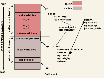
Before continuing, read the following two articles:
Calling Functions
In C programming, when you call a function, the process is abstracted from you, but understanding what happens at the assembly level can be quite insightful. As we have done throughout this module, we will start with a simple example in C, study the corresponding assembly code, and then gradually increase the complexity.
So, let's look at this example of a function calling another function. Note that there are no arguments, nor do either of the functions return a value.
C code:
void addNumbers() {
    int sum = 10 + 32; // The sum is computed but not used since we don't return anything.
}

void myFunction() {
    addNumbers(); // Call addNumbers, but there's no return value to handle.
}
Equivalent Assembly (x86):
.globl addNumbers
addNumbers:
    # Code to compute sum would go here, but since we don't use the result,
    # we can omit it for a void function.
    ret              # Return from addNumbers.

.globl myFunction
myFunction:
    call addNumbers  # Call the addNumbers function.
    # No need to handle a return value since addNumbers is void.
    ret              # Return from myFunction.
The call instruction is used in assembly language to invoke functions. When a call instruction is executed, the CPU does two main things:
- Pushes the address of the next instruction (return address) onto the stack so that the program knows where to return after the function execution.
- Jumps to the target function's starting address to begin execution.
The ret instruction is used in assembly language to return from a procedure or function. When ret is executed, it performs the following actions:
-
Pops the top value from the stack into the instruction pointer register (
EIPon x86 architectures). This value is typically the return address, which was pushed onto the stack by thecallinstruction when the function was initially called. -
Transfers control to the instruction located at the return address, effectively resuming execution at the point immediately after where the function was called.
In summary, the ret instruction is responsible for cleaning up after a function call by restoring the instruction pointer to its previous state, allowing the program to continue executing from where it left off before the function call.
That a simple example. In the next section, we will dive into more complex examples!
Check Your Understanding: For the above example, draw on paper how the stack changes with each instruction execution based on the descriptions of what the instructions do.
Arguments and Result
In x86-64 assembly, the function prologue and epilogue are used to manage the stack frame for a function call, particularly when arguments are being passed and values are being returned. Here's an overview:
Setting up the stack frame (Prologue)
-
Push the base pointer onto the stack to save the previous base pointer value.
push rbp -
Move the stack pointer into the base pointer to set up a new base frame.
mov rbp, rsp -
Allocate space on the stack for local variables by moving the stack pointer.
sub rsp, <size><size>represents the number of bytes needed for local variables.
Cleaning up the stack frame (Epilogue)
-
Move the base pointer back into the stack pointer to deallocate local variables.
mov rsp, rbp -
Pop the old base pointer off the stack to restore the previous base pointer value.
pop rbp -
Return from the function using the
retinstruction.ret
Note: The
leaveinstruction is a shorthand for themovandpopoperations in (in the epilogue) to clean up the stack frame. Essentially,leaveresets the stack pointer and base pointer to their state before the function call.
These steps ensure that each function has its own stack frame, which is essential for local variable management and for the return address to be properly restored when the function completes. Remember that the calling convention may require you to save and restore other registers as well.
Passing Arguments to Functions
Arguments can be passed to functions in a couple of ways:
- Register usage for arguments - In many calling conventions, the first few arguments are passed in registers, which is faster than using the stack. The specific registers used can vary depending on the architecture (e.g., EAX, EDX, ECX on x86; RDI, RSI, RDX, RCX, R8, R9 on x86-64).
- Stack usage for additional arguments - If there are more arguments than there are registers available for argument passing, or if the calling convention dictates, additional arguments are passed on the stack. The stack is also used to pass arguments that are larger than the size of a register.
So, with this information in mind, let's look at an example of a C function call that takes just a few simple arguments:
#include <stdio.h>

// Function declaration
void greet(char *name, int age);

int main() {
    // Function call with arguments
    greet("Alice", 30);

    return 0;
}

// Function definition
void greet(char *name, int age) {
    printf("Hello, %s! You are %d years old.\n", name, age);
}
In this example, the function greet is declared and defined to take two arguments: a string name and an integer age. The main function then calls greet with the arguments "Alice" and 30. When you run this program, it will output: Hello, Alice! You are 30 years old.
Let's look at it as assembly:
section .rodata
helloString db "Hello, %s! You are %d years old.", 10, 0 ; String with a newline and null terminator

section .text
global main
extern printf

; greet function
greet:
    push rbp
    mov rbp, rsp
    sub rsp, 16           ; Allocate space for local variables if needed
    mov rdi, [rbp+16]     ; First argument (char *name)
    mov rsi, [rbp+24]     ; Second argument (int age)
    mov rdx, helloString  ; Address of the format string
    mov rax, 0            ; No vector registers used for floating point
    call printf           ; Call printf function
    leave
    ret

; main function
main:
    push rbp
    mov rbp, rsp
    sub rsp, 16           ; Allocate space for local variables if needed
    mov rdi, name         ; Address of the name string
    mov rsi, 30           ; Age
    call greet            ; Call greet function
    mov eax, 0            ; Return 0
    leave
    ret

section .data
name db "Alice", 0       ; Null-terminated string "Alice"
In this example, the greet function takes two arguments:
- A pointer to a character array (the name string)
- An integer (the age)
Here's how the registers are used in the greet function call:
rdiis used to pass the first argument, which is the pointer to the string"Alice".rsiis used to pass the second argument, which is the integer30.
When calling the printf function from within greet, the arguments are as follows:
rdiis used for the format string.rsiis reused to pass the first variable argument, which is the name string.rdxis used to pass the second variable argument, which is the age integer.raxis set to 0 becauseprintfis a variadic function, andraxis used to indicate the number of vector registers used; in this case, none are used.
The printf function then uses these register values to access the arguments and print the formatted string to the standard output. 🖨️🔢
Return Values from Functions
Values can be returned from a function in a couple of different ways:
-
Return values in registers: For small return values, typically those that are the size of a register or smaller, most calling conventions use registers to return values. On a 64-bit system, the
raxregister is commonly used. Returning values in registers is fast because it avoids the overhead of memory access. 🚀 -
Handling larger return values: When a function needs to return a value larger than the size of a register, such as a large struct or an array, the typical approach is to pass a pointer to a memory space allocated by the caller, where the function can write the return value. This technique is known as passing the return value by reference. The function signature might require the caller to provide a pointer to the space where the return value should be stored. This approach can also be used to return multiple values from a function by passing multiple pointers for each value that needs to be returned.
Here's an example of a function returning a value.
int add(int a, int b) {
    return a + b;
}

int main() {
    int result = add(3, 4);
    return result;
}
Now, let's look at how this might be translated into assembly:
; Function: add
; Adds two integers and returns the result
add:
    mov eax, edi        ; Move first argument (a) into eax
    add eax, esi        ; Add second argument (b) to eax
    ret                 ; Return with result in eax

; Function: main
; Calls add and returns its result
main:
    push rbp            ; Save base pointer
    mov rbp, rsp        ; Set up new base pointer

    mov edi, 3          ; Set first argument (3) for add function
    mov esi, 4          ; Set second argument (4) for add function
    call add            ; Call add function; result will be in eax

    mov ebx, eax        ; Store the result of add in ebx (or another register/memory location)

    mov eax, ebx        ; Move the result into eax to be the return value of main
    pop rbp             ; Restore base pointer
    ret                 ; Return with result in eax
In this Assembly code the main function sets up the stack frame by pushing the base pointer (rbp) onto the stack and then copying the stack pointer (rsp) to rbp. It prepares the arguments for the add function by moving the values 3 and 4 into the edi and esi registers, respectively. The call instruction is used to call the add function. After the call, the result is in the eax register. The result is then moved from eax to ebx for temporary storage (this step is not strictly necessary if you're immediately returning the value). Finally, the result is moved back into eax to set up the return value for main, the stack frame is cleaned up, and the ret instruction is used to return from main.
Check Your Understanding: Implement a simple C program that uses recursion to calculate factorial (e.g., 6! = 6 * 5 * 4 * 3 * 2 * 1). Use your compiler or https://gcc.godbolt.org/ to generate the assembly. Study it and trace through the instructions that are used for modifying stack frame, for passing arguments, and for returning values.
This concludes the explanation for how the computer is able to provide the low-level support for function calls. In the next section, we will dive into a couple of more complex data structures that we commonly use in C: arrays and structures (aka structs).
Arrays
Arrays are fundamental data structures that store elements of the same data type in a contiguous block of memory.
Here a simple example is of an array being declared in C:
int myArray[10]; // Declares an array of 10 integers. The indices range from 0 to 9.
To access the third element, you would use myArray[2] since array indexing starts at 0.
An array uses a single stretch of memory to store all its elements in order to allow for efficient access and manipulation of the array elements. The base address is the memory location of the first element of the array (often denoted as index 0). Array indexing is used to access elements at a particular position within the array. The memory address of any element can be calculated using the base address and the index.
Representing Multi-dimensional Arrays
In order to represent multi-dimensional arrays (like 2D arrays) row-major order is used. This is a method of storing the elements such that the entire first row is stored contiguously, followed by the entire second row, and so on. This is the convention used in languages like C and C++.
Imagine a 2D array with 2 rows and 3 columns:
+-----+-----+-----+
| A00 | A01 | A02 |  <-- Row 0
+-----+-----+-----+
| A10 | A11 | A12 |  <-- Row 1
+-----+-----+-----+
In row-major order, this array would be stored in memory as a single contiguous block like this:
+-----+-----+-----+-----+-----+-----+
| A00 | A01 | A02 | A10 | A11 | A12 |
+-----+-----+-----+-----+-----+-----+
Each cell represents an element of the array, and the elements of each row are stored contiguously before moving on to the next row.
In memory, if the base address is B, and the array is int arr[2][3], the address of the element arr[i][j] (where sizeof(int) is S) can be calculated as:
Address(arr[i][j]) = B + ((i * number_of_columns) + j) * S
For arr[1][2] in our example, the address would be:
Address(arr[1][2]) = B + ((1 * 3) + 2) * S
This calculation ensures that we move past the entire first row (1 * 3 elements) and then to the third element in the second row (+ 2). This representation allows the system to calculate the memory address of any array index extremely efficiently since it relies only on addition and multiplication.
Accessing Array Elements
As is the theme of this module, let's dive into some example C code for accessing array elements and the corresponding assembly code to gain a deeper understanding of how processors work with arrays.
An array name can be thought of as a pointer to its first element, and you can access elements by adding an offset to the pointer. For example, int value = *(myArray + 2); accesses the third element of the array (since it is indexed from 0). This is equivalent to int value = array[2];.
With this in mind, let's write a simple C loop that iterates through all the elements in an array and prints out the values:
for(int i = 0; i < arraySize; i++) {
    printf("%d\n", myArray[i]);
}
Now, let's study the equivalent code in assembly:
mov rax, 0           ; Initialize index to 0
loop_start:
cmp rax, arraySize   ; Compare index with array size
jge loop_end         ; Jump to end if index >= array size
mov rsi, rax         ; Move current index to rsi
mov rdi, myArray     ; Move array base address to rdi
add rdi, rsi         ; Add index to base address
mov rdx, [rdi]       ; Move the value at address to rdx
; Code to print value in rdx
inc rax              ; Increment index
jmp loop_start       ; Jump back to the start of the loop
loop_end:
In this code, the register rax represents the variable i (the loop counter) and the register rdi contains the result of adding the bas address of the array to the index. This register is then used to index into that memory address and store the value of the array element to the register rdx.
Here is another example:
Accessing Multi-dimensional Array Elements
Next, we will look at a slightly more complicated example. This time we will look at working with a 2D array.
Consider the following C code which sues a nested loop to access each element in a 2D array.
for(int i = 0; i < rows; i++) {
    for(int j = 0; j < columns; j++) {
        printf("%d ", myArray[i][j]);
    }
    printf("\n");
}
Notice in the following assembly code how we calculate the offset of the array element using the number of columns in the array. As far as the assembly code is concerned, the data in the array is just a contiguous block of memory.
mov rax, 0          ; Initialize row index to 0
row_loop_start:
cmp rax, rows       ; Compare row index with total rows
jge row_loop_end    ; Jump to end if row index >= rows

mov rbx, 0          ; Initialize column index to 0
column_loop_start:
cmp rbx, columns    ; Compare column index with total columns
jge column_loop_end ; Jump to end if column index >= columns

; Calculate address of myArray[i][j]
mov rsi, rax        ; Move row index to rsi
imul rsi, columns   ; Multiply row index by total columns
add rsi, rbx        ; Add column index to get element index
mov rdi, myArray    ; Move array base address to rdi
lea rdi, [rdi + rsi*4] ; Calculate element address (assuming 4 bytes per int)
mov rdx, [rdi]      ; Move the value at address to rdx
; Code to print value in rdx

inc rbx             ; Increment column index
jmp column_loop_start ; Jump back to the start of the column loop
column_loop_end:

inc rax             ; Increment row index
jmp row_loop_start  ; Jump back to the start of the row loop
row_loop_end:
There are several more topics that we could dive into with regard to working with arrays at the assembly code level including how arrays are passed as function arguments, and how we would maintain arrays of structs. But we haven't talked about structs yet, so let's get right on to that!
Structures
In C programming, a structure (normally referred to as a struct) is a user-defined data type that allows you to combine data items of different kinds. Structures are used to represent a record. Suppose you want to keep track of books in a library. You might want to track the following attributes about each book:
- Title
- Author
- Subject
- Book ID
In C, you can create a structure to hold this information like this:
struct Book {
    char title[50];
    char author[50];
    char subject[100];
    int book_id;
};
To use the struct, you would declare a variable of that type:
struct Book book;
You can then access the members of the structure using the dot . operator:
strcpy(book.title, "C Programming");
strcpy(book.author, "Dennis Ritchie");
strcpy(book.subject, "Programming Language");
book.book_id = 6495407;
Structures can also contain pointers, arrays, and even other structures, making them very versatile for organizing complex data.
How a struct is represented in memory on an x86-64 platform.
Memory Alignment and Padding
Memory alignment is leveraged to improve performance and ensure correctness. Aligned memory accesses are faster because modern CPUs are designed to read or write data at aligned addresses in a single operation. Misaligned accesses may require multiple operations and can lead to penalties in terms of performance.
To ensure proper alignment, compilers often insert unused bytes between structure members, known as padding. This automatic padding helps maintain the correct alignment of each member according to their size and the architecture's requirements, thus preventing misaligned accesses and potential performance hits.
Consider the following C structure:
struct example {
    char a;    // 1 byte
    int b;     // 4 bytes
    char c;    // 1 byte
};
On an x86-64 system, the compiler will likely add padding to align the int b on a 4-byte boundary:
Offset: 0   1   2   3   4   5   6   7
        +---+---+---+---+---+---+---+---+
        | a |   padding | b             |
        +---+---+---+---+---+---+---+---+
        | c |   padding |
        +---+---+---+---+
In this example, 3 bytes of padding are added after char a to align int b, and another 3 bytes are added after char c to make the total size of the structure a multiple of the largest alignment requirement (which is 4 bytes for int in this case).
Accessing Structure Elements in C
You can access elements of a structure using the dot operator if you have a structure variable, or the arrow operator if you have a pointer to a structure. Here's a quick example:
struct Point {
    int x;
    int y;
};

struct Point p1 = {10, 20};
p1.x = 30; // Accessing and modifying using the dot operator

struct Point *p2 = &p1;
p2->y = 40; // Accessing and modifying using the arrow operator
In x86-64 assembly, structures are not explicitly defined. Instead, you work with memory offsets. Assuming the Point structure from above and that it's aligned in memory, you would access its elements by calculating their offsets from the base address of the structure.
Here's how you might do it in assembly, assuming p1 is in the rdi register:
; Assuming p1 is in RDI and it's properly aligned in memory
mov DWORD PTR [rdi], 30   ; Set p1.x to 30. The x offset is 0 because it's the first element.
mov DWORD PTR [rdi+4], 40 ; Set p1.y to 40. Assuming 'int' is 4 bytes, y offset is 4.
Remember that in x86-64, the size of an integer is typically 4 bytes, so you need to account for that when calculating offsets.
Finally, you may remember the linked list data structure from Data Structures and Algorithms. It turns out that structs are an ideal tool for implementing this data structure. Here is a video walking through this example:
Conclusion
We've explored the transformation of basic control flows, delved into the nuances of function calls, and unraveled the complexities of advanced data structures such as arrays and structs. This module has equipped us with a deeper understanding of how our abstract ideas and algorithms that we express using higher-level programming languages are translated into the precise language that our machines comprehend. Next week, we will get into some of the nitty gritty details of how the hardware interprets the instructions and executes them.
Week 3 Participation
During the live class session this week, you will be asked to complete some of the problems that we went through in this material.
Your completion of these questions and answers will make up your Weekly Participation Score.
Assignment 3: Code Bomb Part 2
This lab is from the textbook and supporting material Computer Systems: A Programmer's Perspective. Please visit https://csapp.cs.cmu.edu/3e/labs.html an d refer to the "Bomb Lab" portion for information on completing this lab.
**NOTE: This is Part 1 of 2 parts for this assignment. Complete Phase 4 through 6.
Processor Architecture
We have spent the last couple of weeks diving into machine representation, particularly how higher level programming constructs are represented in assembly code, which can be more directly interpreted by the Central Processing Unit. This week we will get into more details on how those instructions are actually executed by the hardware. To do this, we will review the main components in the processor and how they are constructed using logic gates. We will look at a few examples of basic digital circuits for performing computations (like addition), and then we will see how these digital circuits can be combined to form more complex circuits which are capable of executing the assembly programs we have been learning about. Finally, we will conclude with some concepts around how we can maximize the efficiency of processors.
Note, that we will not be diving extremely deeply into these concepts. Entire courses could be taught in just digital logic design. However, we aim to provide sufficient details that you have a strong idea of the connective tissue ensuring that you have a strong idea of how things work. An understanding of how processors work will aid your overall understanind og how computer systems wok as a whole.
Topics Covered
- Basic Components of a Processor
- Logic Gates and basic digital circuit design
- Combination vs. Sequential circuits and execution
- Clock cycles and clock rate
- Pipelining Overview
Learning Outcomes
After this week, you will be able to:
- Identify and describe the function of the core components within a processor, including the ALU, control unit, registers, and cache.
- Understand and apply the basic principles of digital logic gates in circuit design.
- Differentiate between combinational and sequential circuits and their uses in processor design.
- Define what a clock cycle is and how the clock rate affects processor performance.
- Explain the concept of pipelining and its impact on processor performance and potential issues such as pipeline hazards.
Processor Components
Processor Architecture
The main components of a computer system can be summarized using the following diagram showing four main subsystems: the central processing unit (CPU) made up by the arithmetic logic unit (ALU), the control unit (CU); memory; and input/output (I/O) interfaces. You already know that memory stores instructions that the CPU will execute and data that our programs manipulate. In the following discussion, we will focus on the workings of the CPU.
In order to execute assembly instructions, they must first be in a form that the CPU can interpret, and as we know, CPUs operate on only 1s and 0s. Therefore, the assembly code needs to be further manipulated into a numeric representation, ideally one that allows us to represent programs using a minimal amount of memory.
Instruction Encoding
Earlier in the course, we briefly looked at this showing how assembly code could be equivalently represented as machine code. We will explore that example in more detail.
pushq %rbx
movq %rdx, %rbx
call mult2
movq %rax, (%rbx)
popq %rbx
ret
This assembly code can be equivalently represented as machine code.:
53
48 89 d3
e8 00 00 00 00
48 89 03
5b
c3
If you compare the two programs, you can infer a general idea of what each of the hexadecimal values in the machine code represents. Let's break this down in detail (if you want to double-check the below, you can use the table at http://ref.x86asm.net/, though it is confusing):
-
53: This is a single-byte instruction. The opcode53represents50 + rwhere 50 corresponds to apushoperation and registerrbxis numerically register 3. -
48 89 d348: Prefix indicating an operation involving 64-bit operands.89: Opcode for themovinstruction (on a 16-, 32-, or 64-bit register).d3: Here,d3(1101 0011in binary) breaks down as:11: The first two bits (11) indicate that both operands are registers.010: The next three bits (010) represent the source register (rdx).010: The final three bits (011) represent the destination register (rbx).
-
e8 00 00 00 00e8: Opcode for thecallinstruction.00 00 00 00: This is the displacement for thecallinstruction, which is a relative address. In this case,0x00000000is a placeholder for the memory location of the first instruction for themult2function.
-
48 89 0348: Prefix indicating an operation involving 64-bit operands.89: Opcode for themovinstruction (on a 16-, 32-, or 64-bit register).03: Here,03(0000 0011in binary) breaks down as:00: The first two bits (00) indicate that the destination is a memory address.000: The next three bits (000) represent theraxregister as the source.011: The final three bits (011) represent therbxregister as the base of the memory address.
-
5b: This is a single-byte instruction. The opcode5brepresents58 + rwhere 58 corresponds to apopoperation and registerrbxis numerically register 3 (58 + 3 = 5b in hexadecimal). -
c3: This is a single-byte instruction with the opcodec3for theret(return) command. It pops the return address off the stack and transfers control to that address.
As you can see, each byte or group of bytes in this sequence represents either an opcode (which specifies the operation to be performed), or operands/data (which specify the targets or sources of the operation, such as registers or memory addresses). The combination of opcodes and operands in this sequence of bytes defines the behavior of the CPU when executing this machine code--but how? To understand that, let's start by revisiting the architecture of a processor.
The Fetch-Execute Cycle
We also previously introduced the fetch-execute cycle, the process by which a computer executes instructions in a program.
For convenience, here's the summarized overview of the steps involved in this cycle that we've previously studied:
-
Fetch:
- The CPU fetches the instruction from the computer's memory. This is done by the control unit (CU) which uses the program counter (PC) to keep track of which instruction is next.
- The instruction, stored as a binary code, is retrieved from the memory address indicated by the PC and placed into the Instruction Register (IR).
- The PC is then incremented to point to the next instruction in the sequence, preparing it for the next fetch cycle.
-
Decode:
- The fetched instruction in the IR is decoded by the CU. Decoding involves interpreting what the instruction is and what actions are required to execute it.
- The CU translates the binary code into a set of signals that can be used to carry out the instruction. This often involves determining which parts of the instruction represent the operation code (opcode) and which represent the operand (the data to be processed).
-
Execute:
- The execution of the instruction is carried out by the appropriate component of the CPU. This can involve various parts of the CPU, including the ALU, registers, and I/O controllers.
- If the instruction involves arithmetic or logical operations, the ALU performs these operations on the operands.
- If the instruction involves data transfer (e.g., loading data from memory), the necessary data paths within the CPU are enabled to move data to or from memory or I/O devices.
- Some instructions may require interaction with input/output devices, changes to control registers, or alterations to the program counter (e.g., in the case of a jump instruction).
-
Repeat:
- Once the execution of the instruction is complete, the CPU returns to the fetch step, and the cycle begins again with the next instruction as indicated by the program counter.
To illustrate how the previous example's machine code is executed on a processor, we'll present each step in the fetch-execute cycle in a tabular form.
| Step | Machine Code | Fetch | Decode | Execute | Store | PC Update |
|---|---|---|---|---|---|---|
| 1 | 53 | Fetches 53 from memory at PC. | Decodes 53 as push rbx. | Pushes rbx value onto the stack. | Stack pointer decremented, rbx stored on stack. | PC incremented to point to next instruction (48 89 d3). |
| 2 | 48 89 d3 | Fetches 48 89 d3 from memory at PC. | Decodes 48 89 d3 as mov rdx, rbx. | Moves rdx value to rbx. | rbx updated with rdx value. | PC incremented to point to next instruction (e8 00 00 00 00). |
| 3 | e8 00 00 00 00 | Fetches e8 00 00 00 00 from memory at PC. | Decodes as call with offset 0x0. | Current PC pushed onto stack. Control transferred to address. | Stack pointer decremented, return address stored on stack. | PC updated to target address. |
| 4 | 48 89 03 | Fetches 48 89 03 from memory at PC. | Decodes 48 89 03 as mov rax, (rbx). | Moves rax value to location pointed by rbx. | Memory at rbx address updated with rax value. | PC incremented to point to next instruction (5b). |
| 5 | 5b | Fetches 5b from memory at PC. | Decodes 5b as pop rbx. | Pops top stack value into rbx. | rbx updated with popped value, stack pointer incremented. | PC incremented to point to next instruction (c3). |
| 6 | c3 | Fetches c3 from memory at PC. | Decodes c3 as ret. | Pops return address off the stack, transfers control to that address. | Instruction pointer updated with return address. | PC set to the popped return address, pointing to next instruction in the calling function. |
Each step in the table shows how the Instruction Pointer (or Program Counter) is updated after executing each instruction. The PC points to the next instruction to be executed, and it's updated after each step to reflect the location of the next instruction in the memory. The call instruction is a bit more complex, as it involves storing the return address on the stack and updating the PC to the address of the called function (which in this code is given as a placeholder 0x0). The ret instruction then sets the PC back to the return address, which is the next instruction after the call in the calling function.
Control Unit vs. Arithmetic Logic Unit
From the above example, perhaps you are getting the ide of the distinct bu complementary roles that the Control Unit (CU) and the Arithmetic Logic Unit (ALU) play during the fetch-execute cycle.
The Control Unit orchestrates the overall operation of the processor. Its primary function starts with fetching instructions from the memory, a task guided by the Program Counter (PC). Once an instruction is fetched, the CU decodes it, translating the opcode and operands into a set of actions the CPU understands. This decoding is crucial as it determines how the rest of the processor should respond. The CU then sequences the necessary steps to execute the instruction, ensuring that each phase of the cycle occurs in the correct order and at the right time. It's responsible for managing the flow of data within the CPU, controlling the interactions between various components, including memory, registers, and the ALU.
Additionally, the Control Unit generates and interprets a range of control signals essential for CPU operations. These signals facilitate memory read/write operations, the loading of instruction registers, and more. In cases of branching and conditional instructions, the CU evaluates the conditions and decides the program's execution path, often based on flags set by previous operations.
On the other hand, the Arithmetic Logic Unit is the computational heart of the CPU. It performs all arithmetic operations, such as addition, subtraction, multiplication, and division. Besides arithmetic, the ALU is responsible for executing logical operations like AND, OR, and XOR, which are fundamental in decision-making processes within programs. It compares data, setting flags based on the outcomes, which the CU may use for further decision-making. The ALU also handles operations like bit shifting and rotation, modifying the arrangement of bits within a data word.
The ALU often utilizes internal registers to store temporary data during its operations. Unlike the Control Unit, which directs and orchestrates, the ALU is the executor, carrying out the actual computations and logical decisions as instructed by the decoded operations from the CU.
In essence, the CU and the ALU work in tandem within the CPU: the Control Unit acts as the director, coordinating and controlling the sequence of operations, while the Arithmetic Logic Unit is the performer, executing the computational and logical tasks as instructed.
In order to understand more about how these two main components of the CPU are constructed, we will have to dig deeper.
Digital Logic Design
Before we get into the specifics of microprocessor design, we need to familiarize ourselves with some concepts of digital logic design.
Digital electronics is a vast field, encompassing the principles and techniques used to design and implement electronic circuits and systems that process and manipulate digital signals. Understanding these basics is key to grasping how computers and other digital devices function at the most fundamental level.
In digital circuits, logic levels correspond to the digital values of 0 (low voltage) and 1 (high voltage). Unlike analog signals, which can vary continuously, digital signals switch between fixed logic levels. This characteristic of having discrete values representing discrete states leads to a more robust and noise-resistant form of data transmission, which is required in computing and digital communications.
Introduction Logic Gates
At the heart of digital design are logic gates, the fundamental components that process binary signals.
Imagine logic gates as tiny decision-makers that take in binary inputs where 0 represents "off" or "false," and 1 represents "on" or "true." These gates make logical decisions based on the rules of Boolean algebra.
Each type of logic gate has a specific function and symbol that represents its operation in circuit diagrams (shown below). The output of the logic gate immediately (or nearly immediately) updates when the values on the inputs to the gates change.
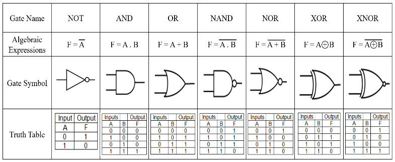
Source: https://www.researchgate.net/figure/Topics-of-basic-logic-gates_fig3_350016075
The AND gate, for instance, outputs a 1 when every input is 1. Conversely, the OR gate outputs a 1 if at least one input is 1. Building on these basics, we have the NAND and NOR gates, which are the negations of the AND and OR gates, respectively.
To predict the behavior of these gates, we use truth tables, which exhaustively list the output for every possible input combination. Boolean expressions, akin to algebraic formulas, provide a compact mathematical representation of the logic gate's function.
Finally, when we visualize these gates in circuit diagrams, we see the flow of logic as it travels through the network of gates, each performing its task to contribute to the overall function of the digital system.
Before continuing, please read Section 3.1 of An Animated Introduction to Digital Logic Design.
Combining Logic Gates
The true power of logic gates is unleashed when we combine them to perform complex operations. This involves using multiple gates in various configurations to realize more complex logical functions. For instance, combining AND, OR, and NOT gates can create a NAND gate, which forms the basis for creating flip-flops, a fundamental component in memory storage and data processing.
A classic example of creating a more complex combinational logic circuit using basic logic gates is the design of a "Half Adder." A Half Adder is a fundamental circuit in digital electronics used to perform the addition of two single-bit binary numbers. It's a great example of how combining simple logic gates can lead to more complex functionalities, such as arithmetic operations.
Half Adder Circuit
The Half Adder circuit takes two single binary digits (bits) as input and produces two outputs: Sum and Carry. The Sum represents the addition result, and the Carry indicates whether there's a carry-out from the addition.
To figure out what the correct combination of logic gates is for the Half Adder, we can construct a truth table. the truth table shows what the different outputs should be based on all the possible combinations of inputs. The truth table for the Half Adder is as follows:
| A (Input) | B (Input) | Sum (S) | Carry (C) |
|---|---|---|---|
| 0 | 0 | 0 | 0 |
| 0 | 1 | 1 | 0 |
| 1 | 0 | 1 | 0 |
| 1 | 1 | 0 | 1 |
Inspection of this truth table will reveal that the the combination of XOR (for the Sum bit) and AND (for the Carry bit) gates effectively handles the binary addition of two single bits, resulting in the following circuit:
Source: https://en.m.wikipedia.org/wiki/Adder_(electronics)#/media/File%3AHalfadder.gif
There are a variety of methods available to digital logic designers to determine and optimize the combination of logic gates that must be used to build more complex circuits, however this is not the focus of this class and we will not go into them. However, if you would like to find out more, read Chapter 2 and 3 of An Animated Introduction to Digital Logic Design.
Combinational vs. Sequential Circuits
Combinational and sequential circuits are two fundamental types of digital circuits used in electronics and computer systems. Here's a concise overview:
Combinational Circuits
Imagine combinational circuits as skilled mathematicians who make decisions based solely on the numbers you provide at that moment. They don't ponder past numbers or anticipate future ones; they focus on the present. This lack of memory elements means their outputs are determined entirely by the current inputs they receive.
Prime examples of combinational circuits are those used in the arithmetic logic unit (ALU) within a CPU. The ALU is a complex, capable of performing a variety of operations such as arithmetic calculations and logical comparisons based on the current inputs, without the need to remember past inputs.
In addition to the Half Adder that we previously discussed, there are some other combinational circuits of illustrative value. One is the single-bit multiplexor (or MUX). A single-bit multiplexer (MUX) is a digital switch that selects one of several input signals and forwards the selected input into a single line. A basic multiplexer has multiple data input lines, one or more control inputs, and one output. In the case of a single-bit 2-to-1 multiplexer, there are two data inputs, one control input, and one output. The control input determines which of the two data inputs is connected to the output.
Here's the truth table for a single-bit 2-to-1 multiplexer:
| Control (C) | Input 0 (I0) | Input 1 (I1) | Output (O) |
|---|---|---|---|
| 0 | 0 | X | 0 |
| 0 | 1 | X | 1 |
| 1 | X | 0 | 0 |
| 1 | X | 1 | 1 |
- Control (C): This is the control input that selects which data input is connected to the output.
- Input 0 (I0) and Input 1 (I1): These are the two data inputs. The output will be one of these inputs, depending on the state of the control input.
- Output (O): This is the output of the multiplexer. The output can be represented logically as
O = (!S . I0) + (S & I1). Using the symbolic representations of logic gates, draw this combinational circuit out on paper and prove to yourself that it implements the above truth table.
In the truth table, 'X' represents a 'don't care' condition, meaning it can be either 0 or 1. The output depends solely on the value of the control input and the corresponding data input line. If the control input is 0, the output is the same as Input 0 (I0); if the control input is 1, the output is the same as Input 1 (I1).
We can also assemble multiple copies of these bit-level circuits to create word-level (i.e., 8-, 16-, 32-, 64-bit versions). You can imagine that as the number of bits increases, the number of logic gates that are necessary to implement the circuit increases rapidly. This is an example of constructing a 64-bit MUX using the single-bit version of the prior example.
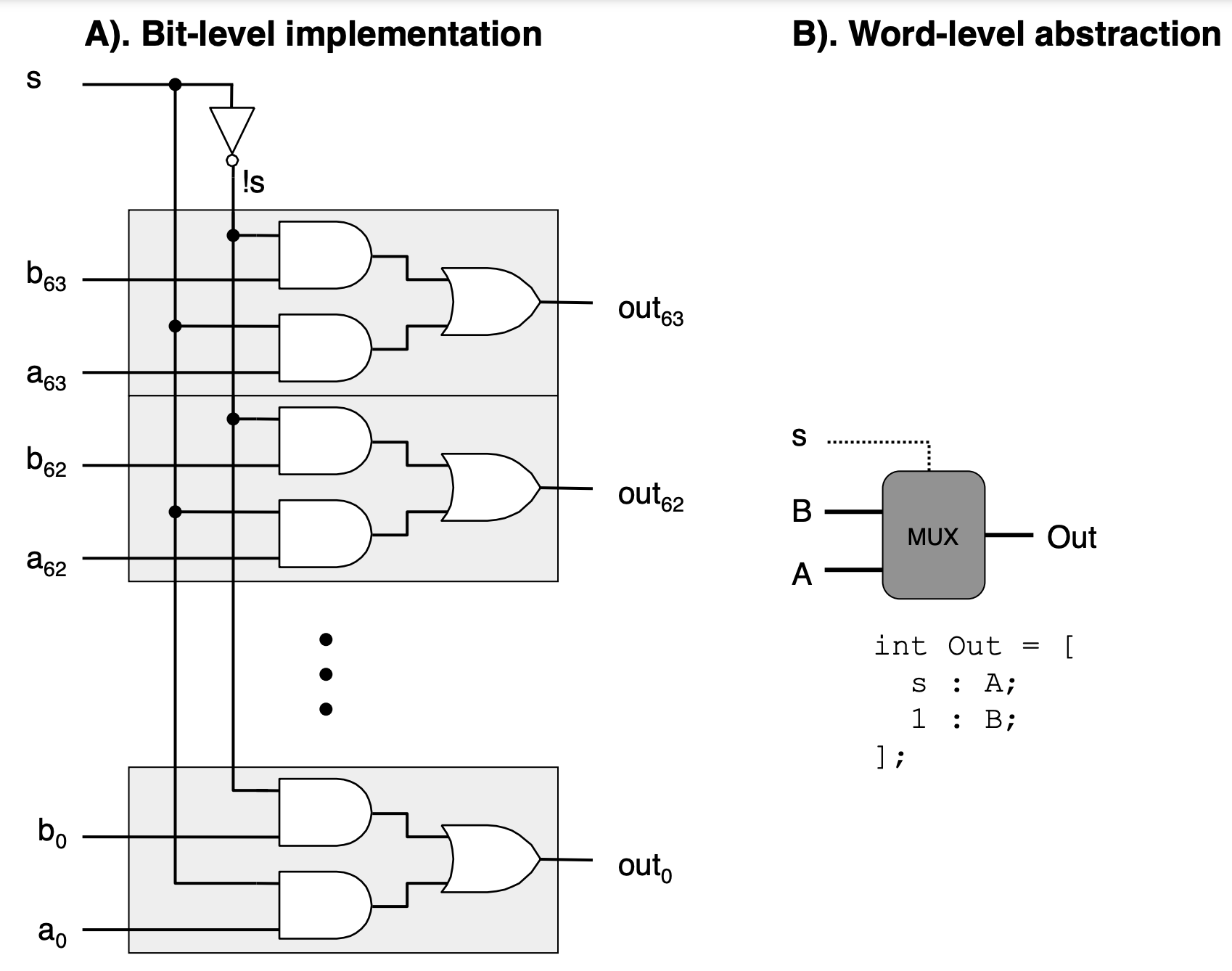
Source: https://csapp.cs.cmu.edu/3e/ics3/arch/logic-word-mux.pdf
Sequential Circuits
The defining characteristic of sequential circuits is their incorporation of memory elements, typically in the form of flip-flops. These memory elements enable the circuits to retain a sense of history, storing the state of past inputs. As a result, the output of a sequential circuit is a reflection of both the current inputs and the accumulated knowledge of previous inputs.
Example: D Flip-Flops
Let's explore the flip-flop circuit in more detail. A D flip-flop, also known as a data or delay flip-flop, is a type of flip-flop that captures the value of the data input (D) at a particular moment in time and outputs this value until the next capture. The capture is controlled by a clock signal (CLK). D flip-flops are widely used for their simplicity and reliability in storing a single bit of data.
- Data Input (D): The input value that is to be stored in the flip-flop.
- Clock Input (CLK): A timing signal that determines when the data input is sampled and transferred to the output.
- Output (Q): The current state of the flip-flop, which holds the last sampled data input.
- Complementary Output (Q'): The inverse of the output (Q), providing the complement of the stored bit.
The behavior of a D flip-flop can be summarized by the following truth table:
| CLK | D | Q (next state) | Q' (next state) |
|---|---|---|---|
| ↑ | 0 | 0 | 1 |
| ↑ | 1 | 1 | 0 |
The CLK column with the upward arrow (↑) indicates that the state change occurs on the rising edge of the clock signal. The D column represents the data input, and the Q and Q' columns show the state of the outputs after the clock edge.
A D flip-flop can be constructed using various logic gates. Here's a basic representation using NAND gates:
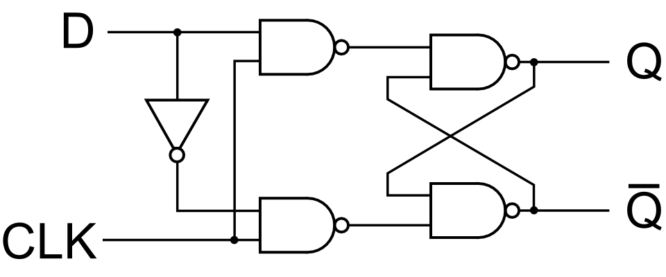
Source: https://electronics.stackexchange.com/questions/497756/what-is-the-relevance-of-a-q-in-the-d-flip-flop-when-using-for-a-memory-module
Check Your Understanding: Take a moment and study this circuit to prove to yourself that it implements the behavior described in the truth table.
In this diagram, the D input is connected to one input of the first NAND gate, while the CLK signal is connected to the other inputs of the NAND gates that control the timing of the data capture. The output Q is fed back into the circuit to maintain the state between clock cycles.
When the clock signal transitions from low to high (rising edge), the value at the D input is "locked in" and appears at the Q output. The Q output will remain in this state until the next rising edge of the clock signal, even if the D input changes in the meantime.
Registers
Registers can be designed with various sizes (8-bit, 16-bit, 32-bit, etc.) by simply increasing the number of D flip-flops and ensuring they are all connected to the same control signals. They are fundamental components in digital systems for holding data, instructions, addresses, and for implementing memory elements and finite state machines.
D flip-flops are combined in parallel to create registers, with each flip-flop responsible for storing one bit of the register's total data capacity. Here's how they are typically combined:
-
Common Clock: All D flip-flops in the register share a common clock signal (CLK). This ensures that each bit is captured simultaneously on the clock's rising or falling edge, depending on the flip-flop's design.
-
Data Inputs: Each D flip-flop has its own data input (D). The binary data to be stored in the register is presented in parallel to these inputs.
-
Outputs: Each flip-flop's output (Q) represents one bit of the register. The outputs of all flip-flops together form the binary data stored in the register.
Here's a simplified representation of an 8-bit register using D flip-flops:
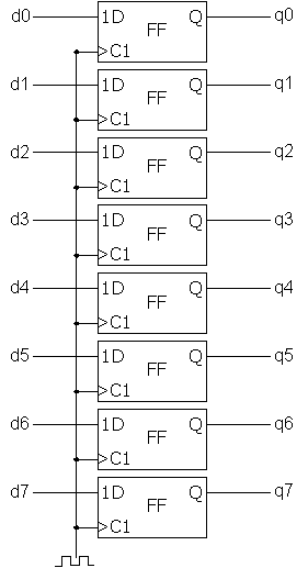
Source: https://commons.wikimedia.org/wiki/File:Register_8bit.png
When the clock signal is pulsed, each flip-flop captures the value present at its D input and holds this value at its Q output until the next clock pulse. This simultaneous capturing of bits across all flip-flops in the register allows for multi-bit data to be stored and manipulated as a single unit.
Summary
This ability to remember gives sequential circuits the power to perform tasks that require an awareness of past events. They are the foundation of devices that need to keep track of progression or store information. Counters, for instance, rely on sequential circuits to tally events over time. Registers serve as temporary storage for data being manipulated by a CPU, holding onto bits and bytes as needed.
Control Unit logic relies heavily on sequential circuits. It uses the stored state information to manage the execution of instructions, coordinate timing, and control data flow. The control unit's ability to remember and act upon a sequence of events is what allows a CPU to execute complex instruction sets efficiently.
Cental Processing Unit Schematic
This is a schematic of a basic CPU (one much simpler than an x86). Now that we have covered how some of these circuits are constructed using logic gates, you should be able to trace what some of the behavior of the CPU might be.
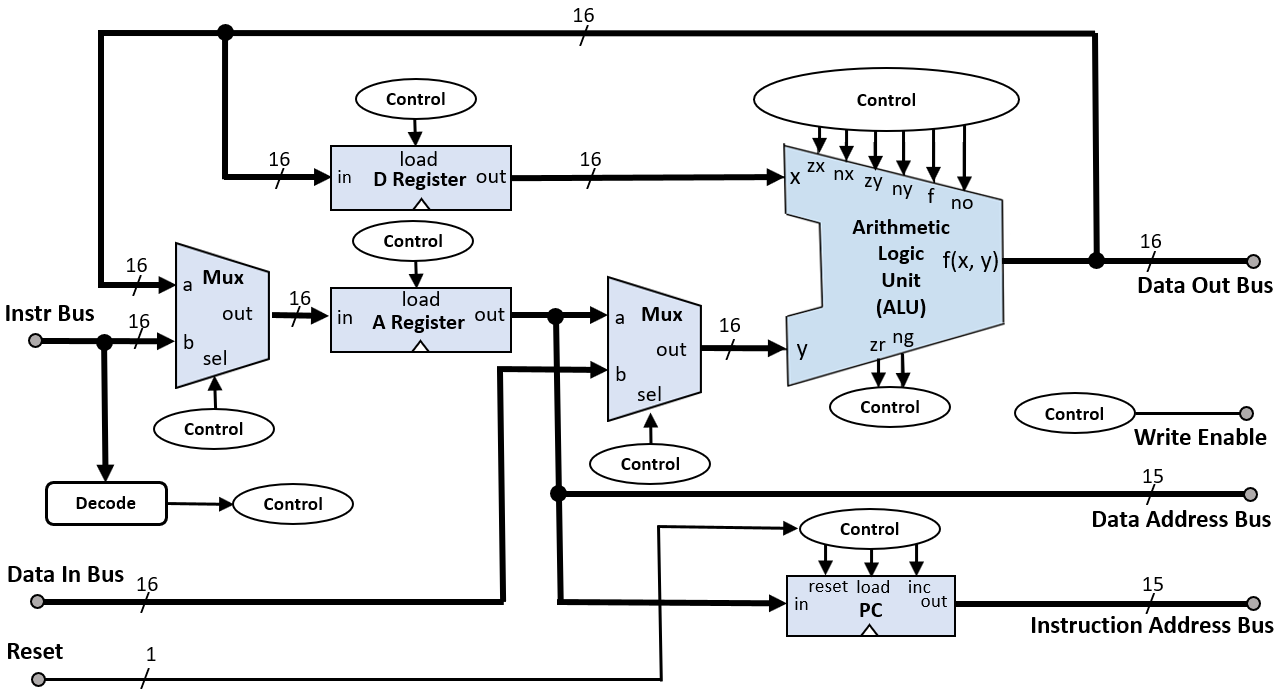
Source: https://en.m.wikipedia.org/wiki/File:Hack_Computer_CPU_Block_Diagram.png
Several key components work together to execute instructions and process data. The central elements typically include multiplexers (muxes) for input selection, registers for data storage, control signals for managing operations, an Arithmetic Logic Unit (ALU) for performing computations, and a program counter (a special register) for tracking the sequence of instructions.
Multiplexers (Muxes): Multiplexers are used to select between different data sources or inputs based on control signals. In this schematic, you can see that muxes are used leading to the 'y' input into the ALU to choose between immediate values provided by an instruction, data from registers, or inputs from I/O devices.
Registers: Registers are small storage units within the CPU that hold data temporarily. They can store operands for the ALU, results of computations, or any data that needs to be quickly accessed by the CPU. Common registers include the accumulator, index registers, stack pointer, and general-purpose registers. Control signals determine when data is loaded into or read from the registers.
Control Signals: Control signals orchestrate the operation of the CPU. They are generated by the control unit based on the current instruction being executed. These signals enable or disable various parts of the CPU, such as telling a register when to capture data, instructing the ALU on which operation to perform, or controlling the flow of data through muxes.
Arithmetic Logic Unit (ALU): The ALU is the computational heart of the CPU, capable of performing arithmetic operations (like addition and subtraction) and logic operations (such as AND, OR, and NOT). It takes operands from registers, processes them according to the control signals, and outputs the result, which can be stored back into a register or used in subsequent operations.
Program Counter (PC): The program counter is a specialized register that keeps track of the address of the next instruction to be executed. After each instruction is fetched, the PC is incremented to point to the following instruction in memory. In some cases, the PC can be modified by control signals to implement jumps or branches in the program flow.
Conclusion
There is one other element that is key to how modern CPUs operate that we haven't spent much time discussing yet. This is the clock signal, which we will discuss next.
Clock Cycles and Clock Rate
Understanding Clock Cycles in CPUs
In processor architecture, clock cycles are the fundamental units of time that dictate the operational tempo of a CPU. A clock cycle is the interval between two consecutive pulses of the CPU's oscillator, which generates a regular clock signal to synchronize the operations of the processor.
Clock Speed
Clock speed, measured in Hertz (Hz), quantifies the number of clock cycles a CPU can perform in one second. A processor with a clock speed of 3 GHz, for example, can execute 3 billion cycles per second. The clock speed is a primary indicator of a processor's raw speed potential; however, it is not the sole determinant of overall performance.
Instruction Execution
Tying into clock speed is the concept of instruction execution. Each CPU instruction may require a varying number of clock cycles to complete, depending on the complexity of the operation and the CPU's architecture. Simple instructions might execute in a single cycle, while complex ones could span multiple cycles. Therefore, the clock speed must be considered alongside the number of cycles required for instruction execution to understand a CPU's efficiency.
IPC (Instructions Per Cycle)
The relationship between clock cycles and instruction execution leads us to the metric of Instructions Per Cycle (IPC). IPC measures the average number of instructions a CPU can execute within a single clock cycle. A high IPC value, when combined with a high clock speed, indicates a processor that can handle a greater volume of instructions in less time, thus delivering superior performance. IPC is a reflection of the processor's architectural efficiency, encompassing factors such as execution pipeline design, caching strategies, and branch prediction.
Multi-core Processors
The concept of IPC becomes even more significant when considering multi-core processors. Each core in a multi-core CPU can execute instructions independently, effectively doubling, tripling, or quadrupling the processing capacity when compared to a single-core CPU. This parallelism allows for more instructions to be processed per clock cycle across the entire CPU, enhancing the throughput and enabling more complex multitasking and parallel processing applications.
Pipelining
Finally, pipelining is a technique that builds upon the principles of clock cycles, instruction execution, and IPC. By breaking down the execution of an instruction into discrete stages—-each of which can be processed in different pipeline stages simultaneously—-a CPU can work on several instructions at once. This means that while one instruction is being executed, another can be decoded, and a third can be fetched, all within the same clock cycle but at different pipeline stages. Pipelining maximizes the use of the CPU's resources, increasing the number of instructions that can be processed in a given time frame and thereby elevating the effective processing power of the CPU.
In summary, the interplay between clock cycles, clock speed, instruction execution, IPC, multi-core processing, and pipelining forms the backbone of CPU performance.
Week 4 Participation
During the live class session this week, you will be asked to complete some of the problems that we went through in this material.
Your completion of these questions and answers will make up your Weekly Participation Score.
Assignment 4: A Simple CPU
For assignment 4, you will spend some time exploring a basic digital logic circuit, and adding additional capability to it ultimately resulting in a basic CPU. For this, we will use the CircuitVerse tool.
The starter circuit ALU that you are provided with is shown below:
This circuit takes two data input bits (A, B) and a carry-in bit (Cin). It produces a data bit (F) and a carry-out bit (Cout)). Two additional control bits (M1 and M0) are required to control what the output of the circuit is: sum, and, or, or xor.
You can change the values of the various inputs by clicking on the corresponding squares. When you do so, the outputs will automatically update. Begin by spending a few minutes exploring this circuit: observe how the output bits change based on the data inputs and the selector bits feeds into the mux. In this assignment, you will apply some of what we have learned this week to expand the circuit.
Getting Started
To get started, follow these steps:
- Click on this link to download the starter template: Download Starter Template.
- Click on this link https://circuitverse.org/groups/7277/invite/m1NNyJ3LM6kg6J4RWj57KbGb to join the CircuitVerse group for our class.
- Click on the Google icon below the login page to login using your Kibo School Google Account.
- On your Circuitverse Dashboard, once you have logged in, click on Launch for Assignment 4. This will create a new workspace that you should complete your work in for this assignment.
- Finally, upload the starter template to your new workspace by using the "Project" -> "Import File" menu option, selecting the file that you downloaded in Step 1, and clicking ok.
Upon creating your project, click on "Help" -> "Tutorial Guide" to get an in-tool guide showing you how to use this tool.
You can click on the varying tabs of the circuit to see some of the sub-components that make up the single-bit ALU: the full adder, which uses two half adders to add two bits; and the 4:1 mux, which allows selecting between one of the four inputs to propagate to the output based on two selection bits.
This tool does not automatically save your work. Be sure to select the option to "Save Online" frequently so that you don't lose your work.
Part 1: Fix the Error (20 pts)
The existing circuit contains a logic error somewhere in it. The logic error may be in the main circuit or one of the the sub-circuits. You have completed this task once the 1-bit ALU produces the correct outputs for all possible inputs.
Part 2: Create an 8 bit ALU (40 pts)
In the second part of the assignment, your task is to create an 8-bit ALU by stringing together multiple single-bit ALUs.
- Click on the "Circuit" menu and selection "New Circuit".
- Call the circuit "8-bit ALU".
- Within the new tab, right-click and select "Insert Sub Circuit" to add new copies of circuits in your workspace. You will need to add 8 copies of the single-bit ALU.
- If you need any additional basic digital logic components, you can search for them in the "Circuit Elements" menu and add them to your design. In particular, you will need multiple copies of the Input and Output pins.
When complete, your 8-bit ALU should have an two 8-bit data inputs (A[7:0] and B[7:0]), an 8 bit data output (O[7:0]), a carry-out bit, and two bit opcode inputs that are used to specifiy what operation the ALU will perform.
Part 3: Build a Mini-CPU (40 pts)
Finally, you are going to use your 8-bit ALU together with some registers and a clock to implement a basic CPU that has 4 operations (add, and, or, and xor), and 4 registers (r0, r1, r2, and r3).
The instruction format will be as follows:
| opcode | src | dest | padding |
|---|---|---|---|
| 2 bits | 2 bits | 2 bits | 00 |
The opcodes are as follows, which you may have observed from the previous parts of the assignment:
| Operation | opcode |
|---|---|
add | 00 |
and | 01 |
or | 10 |
xor | 11 |
The registers are addressed as follows:
| register | address |
|---|---|
r0 | 00 |
r1 | 01 |
r2 | 10 |
r3 | 11 |
So, some example instructions, their binary representation, and are as follows:
| Instruction | Binary representation | Operation |
|---|---|---|
add r0 r2 | 00001000 | r2 = r0 + r2 |
and r1 r3 | 01011100 | r3 = r1 & r3 |
or r2 r2 | 10101000 | r2 = r2 | r2 |
xor r3 r1 | 11110100 | r1 = r3 ^ r1 |
You will create another tab in your workspace to contain the circuit, and along the way to keep things organized, you may want to create additional sub-circuits. You will want to make use of the following components (available within the built-in library) as well:
- D Flip-Flop - This will be useful for building your register. You may note that the D Flip Flop in the library has some additional inputs that we didn't see in our example in the weekly reading. You may want to experiment with it a little bit to understand how they function.
- Button Input - When pressed, emits a 1. When released, emits a 0. This can be used to simulate the clock, which you will need to trigger the updating of values in the registers.
- Multiplexer - For selecting which registers the two inputs of the ALU should be read from.
- Demultiplexer - For selecting which register the output of the ALU should be written to.
The main element missing from this CPU is memory from which instructions would be read. Instead, you'll have to manually configure the inputs for the instruction you want to execute, and trigger the clock to cause the instruction to be executed.
Note: Since our instruction encoding doesn't have any mechanism to provide immediate values or to read values into registers from memory, you may have to manually set values in your register (other than 0) to see that the calculations are working as expected. As a bonus exercise, how could you modify the ISA and the corresponding circuit to support allowing immediate values in the instructions?
Submitting Your Work
Your work must be submitted to Anchor for degree credit and to Gradescope for grading.
- After you have finished designing your circuits using the instructions above, save a images for all of the circuits in your project ("Tools" -> "Download Image" with the options PNG, Full Circuit View, and 1X).
- Export your project using the "Project" -> "Export as File" menu option. This will produce a
.cvfile. - Zip these files into a single zip archive.
- Upload the zip archive to Anchor below.
- Upload your zip archive to Gradescope via the appropriate submission link.
Optimization
Welcome to the Optimization week. You've already learned about Instruction Set Architectures (ISAs) and the basics of processor architecture, which are essential for the next step: writing efficient code. This knowledge isn't just theoretical; it's critical for understanding how processors execute instructions and how this impacts your programming. In this module, we'll explore how to use this understanding to write code that aligns with how CPUs work, optimizing for speed and efficiency.
Optimization is about aligning code with the intricacies of hardware. Different processors have unique ways of handling tasks like branching, pipelining, and memory management. We'll use our understanding of ISAs and CPU architecture to improve algorithms, manage resources, and reduce bottlenecks.
Topics Covered
- Modern processor architecture and its role in optimizing higher-level code.
- Capabilities of compilers and how they optimize
- Loop unrolling
- Reducing procedure calls
- Eliminating memory references
- Branch prediction
- Profiling and use of profilers
- Use of
gprofand Linuxperf
- Use of
Learning Outcomes
After this week, you will be able to:
- Identify performance bottlenecks in a program.
- Utilize performance analysis tools to measure and improve program efficiency.
- Apply optimization techniques like loop unrolling, software pipelining, and loop interchange.
- Understand the impact of memory access patterns on program performance.
Processor Architecture and Optimization
Modern Central Processing Units (CPUs) have become powerhouses of processing capability, thanks to several key features that have been developed to enhance their performance. These features directly impact how software behaves and performs on current-generation systems. A few of these CPU features and how they can influence software performance follows:
- Pipelining: Pipelining in a CPU is a technique where multiple instruction stages (like fetching, decoding, executing) are overlapped and executed in parallel, significantly speeding up processing by handling different parts of multiple instructions simultaneously. This approach increases the instruction throughput, allowing the CPU to work on different stages of several instructions at once, much like an assembly line in a factory.
This video illustrates pipelining on the Intel x86 Haswell architecture.
- Cache Hierarchies: CPUs come with a multi-level cache system (L1, L2, L3) that stores frequently accessed data closer to the processor to reduce latency. A well-optimized cache hierarchy can greatly speed up data access times, improving overall software performance. The following video provides an overview of caches in modern processors.
- Multi-core: Modern CPUs have multiple cores (up to tens of cores), allowing them to perform several tasks simultaneously. This parallel processing capability can significantly boost performance for software that is designed to take advantage of multi-threading. Please watch the following 5 minute portion of this video discussing the evolution of multi-core processors in brief.
- SIMD Instructions (Single Instruction, Multiple Data): These are instructions that can perform the same operation on multiple data points simultaneously. SIMD can greatly accelerate tasks that involve processing large amounts of data, such as graphics rendering or scientific computations.
When software is optimized to utilize these features, it can run more efficiently, handle more tasks at once, and process data faster, leading to a smoother and more responsive user experience.
Next we will provide a high-level view of a wide range of ways that you can try to optimize your code. We will then delve into some of them more deeply, including how the processor architecture is relevant.
Types of Optimizations
The following video is a bit long, but it gives a very nice introduction to a wide variety of different approaches and considerations (with several examples) when working to optimize software. Please take the time to watch it before proceeding.
As you watch this video, keep your ear out for justifications for why the approach is valuable based on computer architectures or how CPUs operate.
Summary
To summarize, and for your future reference, four categories of the "New Bentley Rules" were introduced with each category containing several methods:
- Data Structures
- Packing and Encoding - The idea of packing is to store more than one data value in a machine word. The related idea of encoding is to convert data values in a representation requiring fewer bits.
- Augmentation - Add information to a data structure to make common operations do less work.
- Pre-computation - Perform calculations in advance to avoid doing them at "mission-critical" times.
- Compile-time initialization - Store values of constants during compilation, saving work at execution time.
- Caching - Store results that have been accessed recently so that the program need not compute them again.
- Lazy Evaluation
- Sparsity - Avoid storing and computing on zeroes. ("Fhe fastest way to compute is to not compute at all.")
- Logic
- Constant folding and propagation - Evaluate constant expressions and substitute the result into further expressions, all during compilation.
- Common sub-expression elimination - Avoid computing the same expression multiple times by evaluating the expression once and storing the result for later use.
- Algebraic Identities - Replace expensive algebraic expressions with algebraic equivalents that require less work.
- Short-circuiting - When performing a series of tests, stops evaluation as soon as you know the answer.
- Ordering Tests - In code that executes a sequence of logical tests, perform those are are more often "successful" before tests that are rarely successfully. Similarly, inexpensive tests should precede expensive ones.
- Creating a fast path - Test for simpler cases with less expensive operations, before doing the more complicated cases.
- Combining Tests - Replace a sequence of tests with one test or switch.
- Loops
- Hoisting - avoid recomputing loop-invariant code each time through the body of the loop.
- Sentinels - Leverage special dummy values places in data structure to simplify the logic of boundary conditions and, in particular, the handling of loop-exist tests.
- Loop Unrolling - Attempts to save work by combining several consecutive iterations of a loop into a single iteration, thereby reducing the total number of iterations of the loop and, consequently, the number of times that the instruction that control the loop must be executed.
- Loop Fusion - Combine multiple loops over the same index range into a single loop body, thereby save the overhead of loop control.
- Eliminating Wasted Iterations - Modify loop bounds to avoid executing loop iterations over essentially empty loop bodies.
- Functions
- Inlining - Avoid the overhead of a function call by replacing a call to the function with the body of the function itself.
- Tail-recursion Elimination - Replace a recursive call that occurs as the last step of a function with a branch, saving function-call overhead.
- Coarsening Recursion - Increase the size of the base case and handle it with more efficient code that avoids function-call overhead.
Source: https://ocw.mit.edu/courses/6-172-performance-engineering-of-software-systems-fall-2018/resources/mit6_172f18_lec2/
Note: Premature optimization should be avoided. It can lead to unnecessary complexity in code, making it difficult to read, maintain, and debug. It often involves focusing on performance improvements before fully understanding the system's actual needs and bottlenecks, potentially wasting time optimizing parts of the code that have little impact on overall performance. A better alternative is to first ensure your program is correct, and then devote effort to optimizing the portions of the code that are the largest bottlenecks.
Diving Deep into Optimization
Reading
To dive more deeply into specific optimization techniques, we will rely on a detailed manual that focuses on software optimization. We will then look at a few examples and summarize the key takeaways.
Read the following sections from Optimizing Software in C++: An optimization guide for Windows, Linux, and Mac platforms by Ager Fog, Technical University of Denmark before proceeding. I'll warn you that this is a good amount of reading, so I have included Sherpa links for you to complete after reading each section. Completion of these Sherpa interviews and attendance during the live class session will make up your class participation grades for this week.
- Sections 1.1 and 1.2 - Complete a Sherpa Discussion
- Sections 3.1 and 3.2 - Complete a Sherpa Discussion
- Sections 7.1 through 7.6 - Complete a Sherpa Discussion
- Sections 7.12 through 7.14 - Complete a Sherpa Discussion
- Sections 7.17 through 7.18 - Complete a Sherpa Discussion
- Section 7.20 - Complete a Sherpa Discussion
- Sections 9.1 through 9.6 - Complete a Sherpa Discussion
- Section 9.9 - Complete a Sherpa Discussion
- (Optional) Chapter 14
I encourage you to first skim through the material and try to form some broad generalizations and intuition about the key topics. As you complete the midterm project this week, you will likely want to reference back to these materials so that you can apply the ideas.
Note: The material references examples in C++ though the examples that we will focus on are presented using only features that are also present in the C language, so don't be confused.
Loop Unrolling Example
Loop unrolling is a technique used to increase a program's efficiency by reducing the loop overhead and increasing the loop body's size, allowing for more operations to be executed per iteration. This can lead to better use of CPU caching and instruction pipelining, thus improving overall performance. However, it's important to note that excessive loop unrolling can increase code size and potentially harm performance due to cache misses, so it must be applied judiciously.
C Program Example
Consider a simple program that sums the elements of a large array:
#include <stdio.h>

#define SIZE 10000 // Array size

int main() {
    int array[SIZE];
    int sum = 0;

    // Initialize the array with values
    for(int i = 0; i < SIZE; i++) {
        array[i] = i;
    }

    // Sum the elements of the array
    for(int i = 0; i < SIZE; i++) {
        sum += array[i];
    }

    printf("Sum = %d\n", sum);

    return 0;
}
Optimized Version with Loop Unrolling
In the optimized version, we'll unroll the loop by summing four elements of the array per iteration. This reduces the number of iterations and decreases loop overhead:
#include <stdio.h>

#define SIZE 10000 // Array size, should be a multiple of 4 for this simple example

int main() {
    int array[SIZE];
    int sum = 0;

    // Initialize the array with values
    for(int i = 0; i < SIZE; i++) {
        array[i] = i;
    }

    // Sum the elements of the array with loop unrolling
    for(int i = 0; i < SIZE; i += 4) {
        sum += array[i] + array[i+1] + array[i+2] + array[i+3];
    }

    printf("Sum = %d\n", sum);

    return 0;
}
Key Points
-
Loop Overhead Reduction: Each iteration of the unrolled loop does more work, reducing the total number of loop iterations and, consequently, the loop control overhead.
-
Increased Instruction-Level Parallelism: By executing more operations per iteration, the CPU can better utilize its execution units, potentially leading to performance improvements, especially on modern CPUs with powerful instruction pipelining and execution prediction.
-
Memory Access Optimization: Accessing multiple consecutive array elements in a single loop iteration can improve cache locality, making better use of data loaded into the CPU cache.
There are som considerations, however, including the following:
-
The example assumes the array size (
SIZE) is a multiple of the unroll factor (4 in this case). In real applications, you may need to handle the remainder elements that don't fit neatly into the unrolled loop. -
The benefits of loop unrolling can vary depending on the specific workload, the size of the data being processed, and the architecture of the CPU. It's always a good idea to profile your code to determine whether loop unrolling provides a significant performance boost in your specific case.
Tale Recursion
Tail recursion is a special case of recursion where the recursive call is the last operation in the function. Tail recursion can be optimized by the compiler to reuse the stack frame of the current function call for the next one, effectively converting the recursion into a loop. This optimization can significantly reduce the memory overhead associated with recursive calls and prevent stack overflow for deep recursions.
C Program Example
Consider a simple recursive function to calculate the factorial of a number:
#include <stdio.h>

// Recursive factorial function
unsigned long long factorial(int n) {
    if (n <= 1) return 1; // Base case
    else return n * factorial(n - 1); // Recursive case
}

int main() {
    int number = 20;
    printf("Factorial of %d is %llu\n", number, factorial(number));
    return 0;
}
Optimized Version with Tail Recursion
To optimize this using tail recursion, we introduce an accumulator parameter that carries the result of the factorial calculation through the recursive calls, allowing the final call to return the result directly.
#include <stdio.h>

// Tail recursive factorial function
unsigned long long factorialTail(int n, unsigned long long acc) {
    if (n <= 1) return acc; // Base case
    else return factorialTail(n - 1, n * acc); // Tail recursive case
}

// Wrapper function for factorialTail to provide a clean interface
unsigned long long factorial(int n) {
    return factorialTail(n, 1);
}

int main() {
    int number = 20;
    printf("Factorial of %d is %llu\n", number, factorial(number));
    return 0;
}
Key Points
-
Stack Frame Reuse: The optimized version uses tail recursion, which allows compilers that support tail call optimization (TCO) to reuse the stack frame for each recursive call. This effectively turns the recursive process into an iterative one under the hood, without growing the stack.
-
Preventing Stack Overflow: For very large input values, the original recursive version could lead to a stack overflow error. The tail-recursive version avoids this issue by maintaining a constant stack size through optimization.
-
Maintaining Clean Interfaces: The wrapper function
factorialhides the implementation detail of the accumulator, providing a clean interface to the caller.
It should be noted that tail recursion is most beneficial when the recursion depth can be very large, and there's a risk of stack overflow, or when optimizing for memory usage is crucial.
Data Alignment
Data alignment refers to placing variables in memory at addresses that match their size, which is often a power of two. Proper alignment allows the CPU to access data more efficiently, as misaligned accesses might require multiple memory fetches and can lead to increased cache line usage and potential penalties on some architectures.
Example Demonstrating the Importance of Data Alignment
In this example, we will compare the time it takes to access an aligned vs. a misaligned array of structures.
#include <stdio.h>
#include <stdlib.h>
#include <time.h>

// Aligned struct using manual padding
typedef struct {
    int a;    // 4 bytes on most platforms
    float b;  // 4 bytes
    // Manual padding to align to 16 bytes
    char c[4]; // 4 bytes
    char padding[4]; // Additional padding to make struct size 16 bytes
} AlignedStruct;

// Misaligned struct without specific alignment
typedef struct {
    char x;   // 1 byte
    int a;    // 4 bytes, potentially misaligned depending on 'x' and padding
    float b;  // 4 bytes
    char c[3]; // 3 bytes to ensure misalignment
} MisalignedStruct;

// Function to simulate processing of struct arrays, no change needed
void processStructs(void* structs, size_t count, size_t structSize, int isAligned) {
    clock_t start, end;
    double cpuTimeUsed;
    start = clock();

    // Access logic remains the same as before
    for (size_t i = 0; i < count; i++) {
        char* baseAddr = (char*)structs + i * structSize;
        volatile int a = *((int*)(baseAddr + (isAligned ? 0 : 1))); // Adjust for potential misalignment
        volatile float b = *((float*)(baseAddr + (isAligned ? sizeof(int) : sizeof(int) + 1)));
        volatile char c = *(baseAddr + (isAligned ? sizeof(int) + sizeof(float) : sizeof(int) + sizeof(float) + 1));
    }

    end = clock();
    cpuTimeUsed = ((double) (end - start)) / CLOCKS_PER_SEC;
    printf("Time taken for %s structs: %f seconds\n", isAligned ? "aligned" : "misaligned", cpuTimeUsed);
}

int main() {
    size_t count = 10000000; // Number of struct instances

    // Allocation and processing logic remains unchanged
    AlignedStruct* alignedStructs = (AlignedStruct*)malloc(count * sizeof(AlignedStruct));
    MisalignedStruct* misalignedStructs = (MisalignedStruct*)malloc(count * sizeof(MisalignedStruct));

    processStructs(alignedStructs, count, sizeof(AlignedStruct), 1);
    processStructs(misalignedStructs, count, sizeof(MisalignedStruct), 0);

    free(alignedStructs);
    free(misalignedStructs);

    return 0;
}
Explanation
-
Struct Definitions: Two struct definitions are provided,
AlignedStructandMisalignedStruct.AlignedStructis explicitly aligned to a 16-byte boundary using manual padding, whileMisalignedStructincludes acharat the beginning to simulate misalignment for itsintandfloatmembers. -
Access Function: The
processStructsfunction simulates processing of arrays of both types of structs. It measures and prints the time taken to access elements of each struct in the array. To simulate misalignment effects inMisalignedStruct, the access offsets are adjusted accordingly. -
Performance Measurement: The program measures and compares the time taken to process aligned vs. misaligned struct arrays, highlighting the potential impact of data alignment on performance.
Considerations
-
Compiler and Architecture: The actual performance impact of data alignment can vary significantly across different compilers and target architectures. Some systems handle misalignment with minimal penalties, while others may exhibit a substantial performance degradation.
-
Memory Usage: Aligning data structures can increase memory usage due to added padding. This trade-off between memory usage and access efficiency needs to be considered, especially for memory-constrained environments.
This example demonstrates how data alignment can affect the efficiency of memory access in a C program, emphasizing the importance of considering alignment in performance-critical applications.
Access Data Sequentially
Accessing data sequentially in memory is crucial for optimizing C programs due to the way modern CPUs and memory hierarchies work. Sequential access patterns take advantage of spatial locality, allowing the CPU's cache mechanism to prefetch data efficiently, thereby reducing cache misses and improving overall program speed.
Example: Sum of Array Elements
To demonstrate the importance of accessing data sequentially, let's consider two scenarios where we sum the elements of a 2D array: once accessing the data in a row-major order (sequential access) and once in a column-major order (non-sequential access).
We'll use a large 2D array for this example to ensure that the effects on performance due to caching and access patterns are noticeable.
#include <stdio.h>
#include <stdlib.h>
#include <time.h>

#define ROWS 10000
#define COLS 10000

// Function to sum elements in row-major order
long long sumRowMajor(int arr[ROWS][COLS]) {
    long long sum = 0;
    for (int i = 0; i < ROWS; ++i) {
        for (int j = 0; j < COLS; ++j) {
            sum += arr[i][j];
        }
    }
    return sum;
}

// Function to sum elements in column-major order
long long sumColumnMajor(int arr[ROWS][COLS]) {
    long long sum = 0;
    for (int j = 0; j < COLS; ++j) {
        for (int i = 0; i < ROWS; ++i) {
            sum += arr[i][j];
        }
    }
    return sum;
}

int main() {
    int(*arr)[COLS] = malloc(sizeof(int[ROWS][COLS])); // Dynamic allocation for a large array

    // Initialize array
    for (int i = 0; i < ROWS; ++i) {
        for (int j = 0; j < COLS; ++j) {
            arr[i][j] = 1; // Simplified initialization for demonstration
        }
    }

    clock_t start, end;
    double cpuTimeUsed;

    // Measure time taken for row-major access
    start = clock();
    long long sumRow = sumRowMajor(arr);
    end = clock();
    cpuTimeUsed = ((double) (end - start)) / CLOCKS_PER_SEC;
    printf("Sum (Row-major): %lld, Time: %f seconds\n", sumRow, cpuTimeUsed);

    // Measure time taken for column-major access
    start = clock();
    long long sumCol = sumColumnMajor(arr);
    end = clock();
    cpuTimeUsed = ((double) (end - start)) / CLOCKS_PER_SEC;
    printf("Sum (Column-major): %lld, Time: %f seconds\n", sumCol, cpuTimeUsed);

    free(arr); // Clean up
    return 0;
}
Explanation
-
Row-Major Access: This pattern accesses array elements sequentially as they are stored contiguously in memory, which matches the order of the inner loop. It benefits from spatial locality and prefetching, making it faster.
-
Column-Major Access: This pattern causes more cache misses because it jumps across rows, accessing data that is not contiguous in memory. It results in poorer use of the cache and slower performance due to the higher cost of cache misses.
Expected Outcome
You'll notice that summing the array elements in row-major order is significantly faster than in column-major order due to the efficient use of the CPU cache. Sequential memory access allows the prefetching mechanism to load contiguous memory blocks into the cache ahead of time, reducing the number of cache misses.
Considerations
-
Memory Layout: Understanding the memory layout of data structures is crucial for optimizing memory access patterns. In C, multi-dimensional arrays are stored in row-major order, which influences how to access them optimally.
-
Hardware Specifics: The actual performance gain from sequential access can vary depending on the specific hardware architecture, including the size of the cache lines and the efficiency of the prefetching mechanism.
-
Compiler Optimizations: Modern compilers may attempt to optimize non-sequential accesses in some cases, but it's generally best to manually ensure data is accessed sequentially whenever possible for critical performance paths.
Summary
Optimizing C programs for efficiency involves understanding low-level details of how a CPU processes instructions and how caching and memory access impact CPU performance, among other things. Proper data alignment reduces memory access penalties and enhances cache utilization, while tail recursion optimization can significantly decrease stack usage, transforming recursive calls into more efficient loops. Sequential data access takes advantage of CPU cache prefetching, minimizing cache misses and improving program execution speed by ensuring memory reads and writes are predictable and contiguous.
Profiling
Using a profiler in C programming is an essential skill for developers looking to optimize their applications for better performance. A profiler helps identify the parts of a program that consume the most resources, such as CPU time or memory usage. By pinpointing these hotspots, developers can focus their optimization efforts where they will have the most significant impact, rather than blindly trying to optimize the entire codebase. This targeted approach not only saves time but also leads to more efficient and faster-running applications.
This video introduces a couple of common profiling tools used in C:
To start using a profiler, one must first choose the right tool for their needs. There are various profilers available for C, ranging from gprof, a GNU profiler that comes with the GCC compiler, to more sophisticated tools like Valgrind and Google's gperftools. Each profiler has its strengths and suits different types of applications and profiling needs. For instance, gprof is great for getting a general overview of where a program spends its time, while Valgrind's Callgrind tool offers detailed information about cache usage and branch prediction statistics.
After selecting a suitable profiler, the next step involves instrumenting the code, if necessary, and running the profiler. This process typically starts by compiling the C program with specific flags to enable profiling, such as -pg for gprof. Then, the program is run as usual, and the profiler generates a report detailing the program's execution. This report can show various metrics, including function call counts, execution time spent in each function, and memory usage patterns. The level of detail and the metrics provided depend on the profiler's capabilities.
Interpreting the profiler's report is crucial for effective optimization. Developers should look for functions with high execution times or those called excessively as starting points for optimization. It's also important to pay attention to memory usage patterns, as inefficient memory access can significantly impact performance due to cache misses. Armed with this information, developers can refactor code, optimize algorithms, or apply specific techniques like loop unrolling or data alignment to address the identified bottlenecks. Ultimately, iterative profiling and optimization based on profiler feedback can lead to highly optimized and efficient C applications.
Weeks 5 and 6 Participation
During the live class sessions this week and next, you will be asked to complete some of the problems that we went through in this material.
Your completion of these questions and answers will make up your Weekly Participation Score.
Week 5
This week for your participation, we will be using a new tool that will ask you questions about a couple of different topics.
-
Mid-point Course Reflection - Write a 1 paragraph summary of your experience in the course thus far this term. You will then be asked additional questions about that experience.
-
Use of the Stack Frame - This will ask you some questions based on your reading this week.
Week 6
For the Week 6 participation score, your grade will be determined by the completion of the Sherpa Discussions associated with your reading assignment and by your live class attendance:
Read the following sections from Optimizing Software in C++: An optimization guide for Windows, Linux, and Mac platforms by Ager Fog, Technical University of Denmark before proceeding. I'll warn you that this is a good amount of reading, so I have included Sherpa links for you to complete after reading each section. Completion of these Sherpa interviews and attendance during the live class session will make up your class participation grades for this week.
- Sections 1.1 and 1.2 - Complete a Sherpa Discussion
- Sections 3.1 and 3.2 - Complete a Sherpa Discussion
- Sections 7.1 through 7.6 - Complete a Sherpa Discussion
- Sections 7.12 through 7.14 - Complete a Sherpa Discussion
- Sections 7.17 through 7.18 - Complete a Sherpa Discussion
- Section 7.20 - Complete a Sherpa Discussion
- Sections 9.1 through 9.6 - Complete a Sherpa Discussion
Midterm Project - Performance
This performance assignment is based on the one by Bryant and O’Hallaron for Computer Systems: A Programmer’s Perspective, Third Edition. Please visit https://csapp.cs.cmu.edu/3e/labs.html an d refer to the "Performance Lab" portion for information on completing this lab.
This lab was further enhanced by Matthew Flatt at University of Utah (https://my.eng.utah.edu/~cs4400/performance.html)
Week 7 Participation
For your participation points this week, during class, you will provide status updates on each of your assignments and your midterm projects. For work that is incomplete, you will identify blockers and decide upon next steps to ensure forward progress on your work.
We will collect this information via a Gradescope submission, which will only be available during the class time.
The Memory Hierarchy
This module builds on the foundation laid in previous modules on processor architecture and program optimization. It explores memory technologies, such as SRAM and DRAM, non-volatile storage, and the principles of memory hierarchy, including the locality principle and cache operation. The module delves into the design and implementation of caches, addressing direct-mapped and associative caches, block size, cache conflicts, and write strategies. This module is crucial for understanding how efficient memory usage can significantly impact system performance.
Topics Covered
- Technologies
- Locality
- Caches and Caching Strategies
- Writing cache-friendly Code
Learning Outcomes
After this week, you will be able to:
- Describe the different levels of the memory hierarchy and their characteristics.
- Analyze cache organization and mapping techniques (e.g., direct-mapped, set-associative, fully associative).
- Explain the principles of virtual memory and its role in address space management.
- Evaluate the trade-offs between memory hierarchy levels in terms of speed, capacity, and cost.
The content in this module is taken from MIT Open Courseware. Full video lectures of this material is available from https://ocw.mit.edu/courses/6-004-computation-structures-spring-2017/pages/c14/c14s2/.
Chris Terman. 6.004: Computation Structures. Spring 2017. Massachusetts Institute of Technology: MIT OpenCouseWare, https://ocw.mit.edu/. License: Creative Commons BY-NC-SA.
Memory Technologies
In past weeks we completed the design of a very simple microprocessor and learned about the overall architecture of a much more complicated microprocessor. One of the major limitations of our microprocessor is that it didn't interact with memory in any way. However, we know that the execution of every instructions starts by fetching the instruction from main memory. And ultimately all the data processed by the CPU is loaded from or stored to main memory. A very few frequently-used variable values can be kept in the CPU’s register file, but most interesting programs manipulate much more data than can be accommodated by the storage available as part of the CPU datapath.
In fact, the performance of most modern computers is limited by the bandwidth, i.e., bytes/second, of the connection between the CPU and main memory, the so-called memory bottleneck. The goal of this module is to understand the nature of the bottleneck and to see if there are architectural improvements we might make to minimize the problem as much as possible.
We have a number of memory technologies at our disposal, varying widely in their capacity, latency, bandwidth, energy efficiency and their cost. Not surprisingly, we find that each is useful for different applications in our overall system architecture.
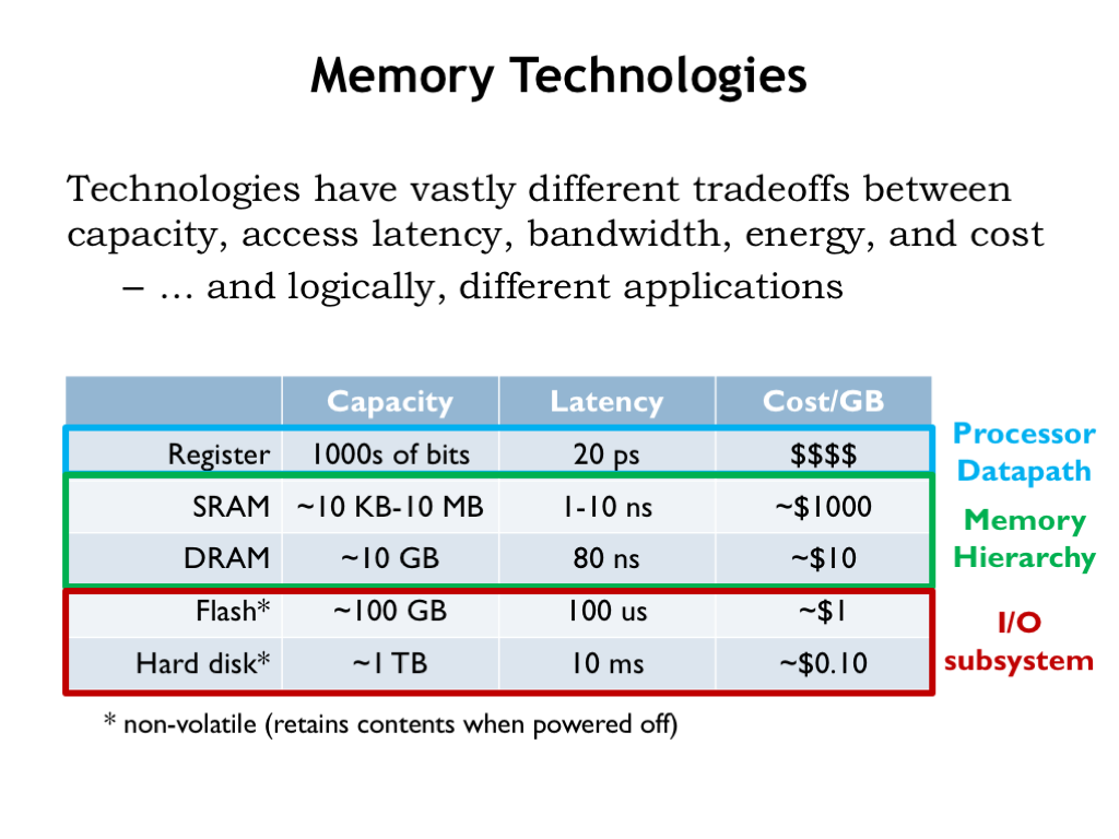
Our registers are built from sequential logic and provide very low latency access (20ps or so) to at most a few thousands of bits of data. Static and dynamic memories, which we’ll discuss further, offer larger capacities at the cost of longer access latencies. Static random-access memories (SRAMs) are designed to provide low latencies (a few nanoseconds at most) to many thousands of locations. Already we see that more locations means longer access latencies — this is a fundamental size vs. performance tradeoff of our current memory architectures. The tradeoff comes about because increasing the number of bits will increase the area needed for the memory circuitry, which will in turn lead to longer signal lines and slower circuit performance due to increased capacitive loads.
Dynamic random-access memories (DRAMs) are optimized for capacity and low cost, sacrificing access latency. As we’ll see, we can use both SRAMs and DRAMs to build a hybrid memory hierarchy that provides low average latency and high capacity — an attempt to get the best of both worlds!
Notice that the word “average” has snuck into the performance claims. This means that we’ll be relying on statistical properties of memory accesses to achieve our goals of low latency and high capacity. In the worst case, we’ll still be stuck with the capacity limitations of SRAMs and the long latencies of DRAMs, but we’ll work hard to ensure that the worst case occurs infrequently!
Flash memory and hard-disk drives provide non-volatile storage. Non-volatile means that the memory contents are preserved even when the power is turned off. Hard disks are at the bottom of the memory hierarchy, providing massive amounts of long-term storage for very little cost. Flash memories, with a 100-fold improvement in access latency, are often used in concert with hard-disk drives in the same way that SRAMs are used in concert with DRAMs, i.e., to provide a hybrid system for non-volatile storage that has improved latency and high capacity.
Let’s learn a bit more about each of these four memory technologies, then we’ll return to the job of building our memory system.
Static RAM
Static RAMs (SRAMs) are organized as an array of memory locations, where a memory access is either reading or writing all the bits in a single location. Here we see the component layout for a 8-location SRAM array where each location holds 6 bits of data. You can see that the individual bit cells are organized as 8 rows (one row per location) by 6 columns (one column per bit in each memory word). The circuitry around the periphery is used to decode addresses and support read and write operations.
To access the SRAM, we need to provide enough address bits to uniquely specify the location. In this case we need 3 address bits to select one of the 8 memory locations. The address decoder logic sets one of the 8 wordlines (the horizontal wires in the array) high to enable a particular row (location) for the upcoming access. The remaining wordlines are set low, disabling the cells they control. The active wordline enables each of the SRAM bit cells on the selected row, connecting each cell to a pair of bit lines (the vertical wires in the array). During read operations the bit lines carry the analog signals from the enabled bit cells to the sense amplifiers, which convert the analog signals to digital data. During write operations incoming data is driven onto the bit lines to be stored into the enabled bit cells.
Larger SRAMs will have a more complex organization in order to minimize the length, and hence the capacitance, of the bit lines.
This video provides details about how we read from and write to SRAM:
In summary, the circuitry for the SRAM is organized as an array of bit cells, with one row for each memory location and one column for each bit in a location. Each bit is stored by two inverters connected to form a bistable storage element. Reads and writes are essentially analog operations performed via the bitlines and access FETs.
DRAM
The SRAM uses 6 MOSFETs for each bit cell. Can we do better? What’s the minimum number of MOSFETs needed to store a single bit of information?
NOTE: A MOSFET (Metal-Oxide-Semiconductor Field-Effect Transistor) cell is a type of transistor used for amplifying or switching electronic signals.. It consists of a gate, source, and drain terminals; the gate terminal controls the conductivity between the source and drain by applying a voltage, which modulates the current flow. MOSFETs are fundamental components in integrated circuits, widely used in digital and analog circuits due to their high efficiency and fast switching speeds.
Well, we’ll need at least one MOSFET so we can select which bits will be affected by read and write operations. We can use a simple capacitor for storage, where the value of a stored bit is represented by voltage across the plates of the capacitor. The resulting circuit is termed a dynamic random-access memory (DRAM) cell.
If the capacitor voltage exceeds a certain threshold, we’re storing a 1 bit, otherwise we’re storing a 0. The amount of charge on the capacitor, which determines the speed and reliability of reading the stored value, is proportional to the capacitance. We can increase the capacitance by increasing the dielectric constant of the insulating material between the two plates of the capacitor, increasing the area of the plates, or by decreasing the the distance between the plates. All of these are constantly being improved.
A cross section of a modern DRAM cell is shown here. The capacitor is formed in a large trench dug into the substrate material of the integrated circuit. Increasing the depth of the trench will increase the area of the capacitor plates without increasing the cell’s area. A very thin insulating layer separates the outer plate from the inner plate, which is connected to some reference voltage (shown as GND in this diagram).All
All this is to say that the resulting circuit is quite compact: about 20-times less area/bit than an SRAM bit cell. There are some challenges however. There’s no circuitry to manage the static charge on the capacitor, so stored charge will leak from the outer plate of the capacitor, hence the name dynamic memory. This limits the amount of time we can leave the capacitor unattended and still expect to read the stored value. This means we’ll have to arrange to read then re-write each bit cell (called a refresh cycle) every 10ms or so, adding to the complexity of the DRAM interface circuitry.
This video provides details about how we read from and write to DRAM:
Check Your Understanding: Some new terms were probably used in the explanation of what makes up DRAM and how it is used. On a piece of paper list out those terms and spend a few minutes doing independent researching using Google or ChatGPT to gain a better understanding of those terms.
In summary, DRAM bit cells consist of a single access FET connected to a storage capacitor that’s cleverly constructed to take up as little area as possible. DRAMs must rewrite the contents of bit cells after they are read and every cell must be read and written periodically to ensure that the stored charge is refreshed before it’s corrupted by leakage currents.
DRAMs have much higher capacities than SRAMs because of the small size of the DRAM bit cells, but the complexity of the DRAM interface circuitry means that the initial access to a row of locations is quite a bit slower than an SRAM access. However subsequent accesses to the same row happen at speeds close to that of SRAM accesses.
Both SRAMs and DRAMs will store values as long as their circuitry has power. But if the circuitry is powered down, the stored bits will be lost. For long-term storage we will need to use non-volatile memory technologies, the topic of the next lecture segment.
Non-volatile Storage
Non-volatile memories are used to maintain system state even when the system is powered down.
Flash Memory
One example of non-volatile memory is flash memory. In flash memories, long-term storage is achieved by storing charge on an well-insulated conductor called a floating gate, where it will remain stable for years. The floating gate is incorporated in a standard MOSFET, placed between the MOSFET’s gate and the MOSFET’s channel. If there is no charge stored on the floating gate, the MOSFET can be turned on, i.e., be made to conduct, by placing a voltage on the gate terminal, creating an inversion layer that connects the MOSFET’s source and drain terminals. If there is a charge stored on the floating gate, a higher voltage is required to turn on the MOSFET. By setting the gate terminal to a voltage between and , we can determine if the floating gate is charged by testing to see if the MOSFET is conducting.
In fact, if we can measure the current flowing through the MOSFET, we can determine how much charge is stored on the floating gate, making it possible to store multiple bits of information in one flash cell by varying the amount of charge on its floating gate. Flash cells can be connected in parallel or series to form circuits resembling CMOS NOR or NAND gates, allowing for a variety of access architectures suitable for either random or sequential access.
Flash memories are very dense, approaching the areal density of DRAMs, particularly when each cell holds multiple bits of information.
Read access times for NOR flash memories are similar to that of DRAMs, several tens of nanoseconds. Read times for NAND flash memories are much longer, on the order of 10 microseconds. Write times for all types of flash memories are quite long since high voltages have to be used to force electrons to cross the insulating barrier surrounding the floating gate.
Flash memories can only be written some number of times before the insulating layer is damaged to the point that the floating gate will no longer reliably store charge. Currently the number of guaranteed writes varies between 100,000 and 1,000,000. To work around this limitation, flash chips contain clever address mapping algorithms so that writes to the same address actually are mapped to different flash cells on each successive write.
The bottom line is that flash memories are a higher-performance but higher-cost replacement for the hard-disk drive, the long-time technology of choice for non-volatile storage.
Hard Disk Drives (HDDs)
A hard-disk drive (HDD) contains one or more rotating platters coated with a magnetic material. The platters rotate at speeds ranging from 5400 to 15000 RPM. A read/write head positioned above the surface of a platter can detect or change the orientation of the magnetization of the magnetic material below. The read/write head is mounted on an actuator that allows it to be positioned over different circular tracks.
To read a particular sector of data, the head must be positioned radially over the correct track, then wait for the platter to rotate until it’s over the desired sector. The average total time required to correctly position the head is on the order of 10 milliseconds, so hard disk access times are quite long.
However, once the read/write head is in the correct position, data can be transferred at the respectable rate of 100 megabytes/second. If the head has to be repositioned between each access, the effective transfer rate drops 1000-fold, limited by the time it takes to reposition the head.
Hard disk drives provide cost-effective non-volatile storage for terabytes of data, albeit at the cost of slow access times.
Summary
This completes our whirlwind tour of memory technologies. If you’d like to learn a bit more, Wikipedia has useful articles on each type of device. SRAM sizes and access times have kept pace with the improvements in the size and speed of integrated circuits. Interestingly, although capacities and transfer rates for DRAMs and HDDs have improved, their initial access times have not improved nearly as rapidly. Thankfully over the past decade flash memories have helped to fill the performance gap between processor speeds and HDDs. But the gap between processor cycle times and DRAM access times has continued to widen, increasing the challenge of designing low-latency high-capacity memory systems.
The capacity of the available memory technologies varies over 10 orders of magnitude, and the variation in latencies varies over 8 orders of magnitude. This creates a considerable challenge in figuring out how to navigate the speed vs. size tradeoffs.
The Memory Hierarchy
Each transition in memory hierarchy shows the same fundamental design choice: we can pick smaller-and-faster or larger-and-slower. This is a bit awkward actually — can we figure how to get the best of both worlds?
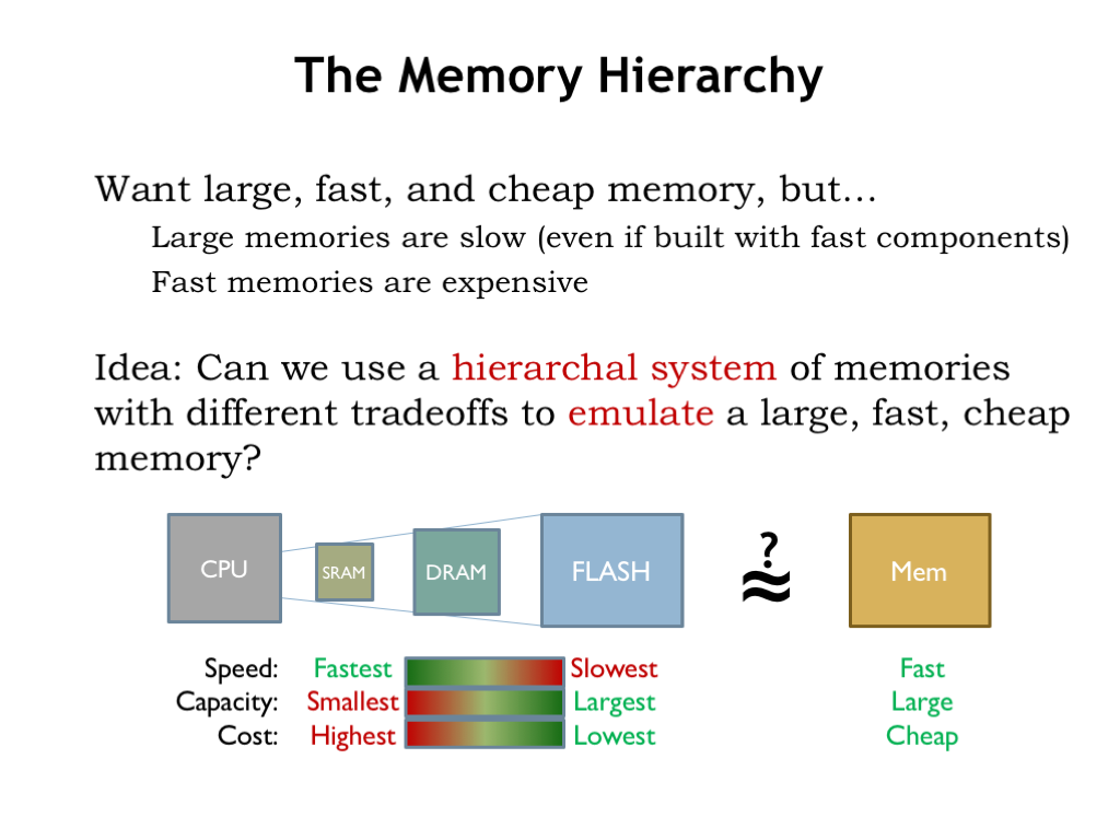
We want our system to behave as if it had a large, fast, and cheap main memory. Clearly we can’t achieve this goal using any single memory technology.
Here’s an idea: can we use a hierarchical system of memories with different tradeoffs to achieve close to the same results as a large, fast, cheap memory? Could we arrange for memory locations we’re using often to be stored, say, in SRAM and have those accesses be low latency? Could the rest of the data could be stored in the larger and slower memory components, moving the between the levels when necessary? Let’s follow this train of thought and see where it leads us.
There are two approaches we might take. The first is to expose the hierarchy, providing some amount of each type of storage and let the programmer decide how best to allocate the various memory resources for each particular computation. The programmer would write code that moved data into fast storage when appropriate, then back to the larger and slower memories when low-latency access was no longer required. There would only be a small amount of the fastest memory, so data would be constantly in motion as the focus of the computation changed.
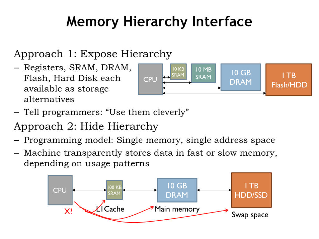
This approach has had notable advocates. Perhaps the most influential was Seymour Cray, the “Steve Jobs” of supercomputers. Cray was the architect of the world’s fastest computers in each of three decades, inventing many of the technologies that form the foundation of high-performance computing. His insight to managing the memory hierarchy was to organize data as vectors and move vectors in and out of fast memory under program control. This was actually a good data abstraction for certain types of scientific computing and his vector machines had the top computing benchmarks for many years.
The second alternative is to hide the hierarchy and simply tell the programmer they have a large, uniform address space to use as they wish. The memory system would, behind the scenes, move data between the various levels of the memory hierarchy, depending on the usage patterns it detected. This would require circuitry to examine each memory access issued by the CPU to determine where in the hierarchy to find the requested location. And then, if a particular region of addresses was frequently accessed — say, when fetching instructions in a loop — the memory system would arrange for those accesses to be mapped to the fastest memory component and automatically move the loop instructions there. All of this machinery would be transparent to the programmer: the program would simply fetch instructions and access data and the memory system would handle the rest.
Could the memory system automatically arrange for the right data to be in the right place at the right time? Cray was deeply skeptical of this approach. He famously quipped “that you can’t fake what you haven’t got”. Wouldn’t the programmer, with her knowledge of how data was going to be used by a particular program, be able to do a better job by explicitly managing the memory hierarchy?
The Locality Principle
It turns out that when running general-purpose programs, it is possible to build an automatically managed, low-latency, high-capacity hierarchical memory system that appears as one large, uniform memory. What’s the insight that makes this possible? That’s the topic of the next section.
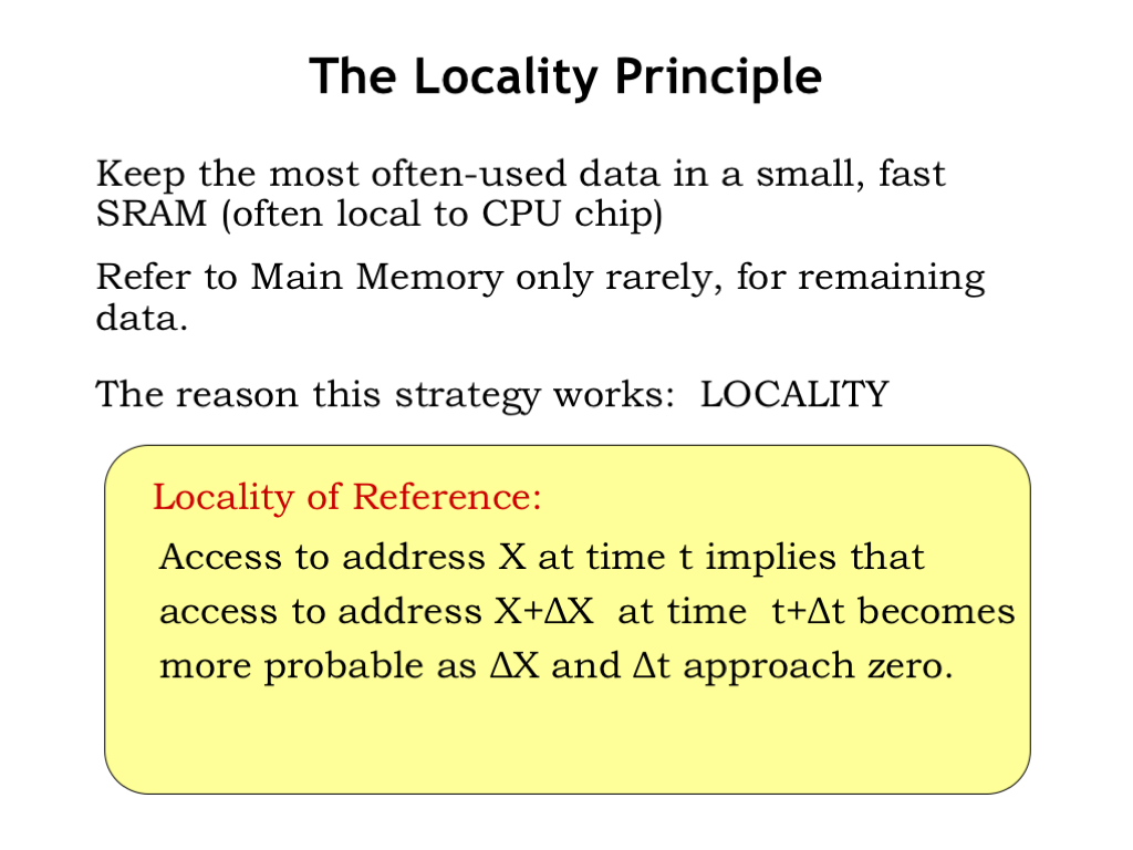
So, how can the memory system arrange for the right data to be in the right place at the right time? Our goal is to have the frequently-used data in some fast SRAM. That means the memory system will have to be able to predict which memory locations will be accessed. And to keep the overhead of moving data into and out of SRAM manageable, we’d like to amortize the cost of the move over many accesses. In other words we want any block of data we move into SRAM to be accessed many times.
When not in SRAM, data would live in the larger, slower DRAM that serves as main memory. If the system is working as planned, DRAM accesses would happen infrequently, e.g., only when it’s time to bring another block of data into SRAM.
If we look at how programs access memory, it turns out we can make accurate predictions about which memory locations will be accessed. The guiding principle is locality of reference which tells us that if there’s an access to address X at time t, it’s very probable that the program will access a nearby location in the near future.
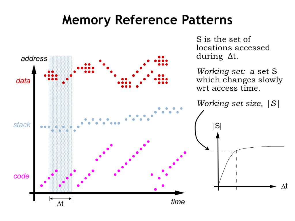
To understand why programs exhibit locality of reference, let’s look at how a running program accesses memory.
Instruction fetches are quite predictable. Execution usually proceeds sequentially since most of the time the next instruction is fetched from the location after that of the current instruction. Code that loops will repeatedly fetch the same sequence of instructions, as shown here on the left of the time line. There will of course be branches and subroutine calls that interrupt sequential execution, but then we’re back to fetching instructions from consecutive locations. Some programming constructs, e.g., method dispatch in object-oriented languages, can produce scattered references to very short code sequences (as shown on the right of the time line) but order is quickly restored.
This agrees with our intuition about program execution. For example, once we execute the first instruction of a procedure, we’ll almost certainly execute the remaining instructions in the procedure. So if we arranged for all the code of a procedure to moved to SRAM when the procedure’s first instruction was fetched, we’d expect that many subsequent instruction fetches could be satisfied by the SRAM. And although fetching the first word of a block from DRAM has relatively long latency, the DRAM’s fast column accesses will quickly stream the remaining words from sequential addresses. This will amortize the cost of the initial access over the whole sequence of transfers.
The story is similar for accesses by a procedure to its arguments and local variables in the current stack frame. Again there will be many accesses to a small region of memory during the span of time we’re executing the procedure’s code.
Data accesses generated by LD and ST instructions also exhibit locality. The program may be accessing the components of an object or struct. Or it may be stepping through the elements of an array. Sometimes information is moved from one array or data object to another, as shown by the data accesses on the right of the timeline.
Using simulations we can estimate the number of different locations that will be accessed over a particular span of time. What we discover when we do this is the notion of a working set of locations that are accessed repeatedly. If we plot the size of the working set as a function of the size of the time interval, we see that the size of the working set levels off. In other words once the time interval reaches a certain size the number of locations accessed is approximately the same independent of when in time the interval occurs.
As we see in our plot to the left, the actual addresses accessed will change, but the number of different addresses during the time interval will, on the average, remain relatively constant and, surprisingly, not all that large!
This means that if we can arrange for our SRAM to be large enough to hold the working set of the program, most accesses will be able to be satisfied by the SRAM. We’ll occasionally have to move new data into the SRAM and old data back to DRAM, but the DRAM access will occur less frequently than SRAM accesses.You can see that thanks to locality of reference we’re on track to build a memory out of a combination of SRAM and DRAM that performs like an SRAM but has the capacity of the DRAM.
Caches
The SRAM component of our hierarchical memory system is called a cache. It provides low-latency access to recently-accessed blocks of data. If the requested data is in the cache, we have a cache hit and the data is supplied by the SRAM.
If the requested data is not in the cache, we have a cache miss and a block of data containing the requested location will have to be moved from DRAM into the cache. The locality principle tells us that we should expect cache hits to occur much more frequently than cache misses.
Modern computer systems often use multiple levels of SRAM caches. The levels closest to the CPU are smaller but very fast, while the levels further away from the CPU are larger and hence slower. A miss at one level of the cache generates an access to the next level, and so on until a DRAM access is needed to satisfy the initial request.
Caching is used in many applications to speed up access to frequently-accessed data. For example, your browser maintains a cache of frequently-accessed web pages and uses its local copy of the web page if it determines the data is still valid, avoiding the delay of transferring the data over the Internet.
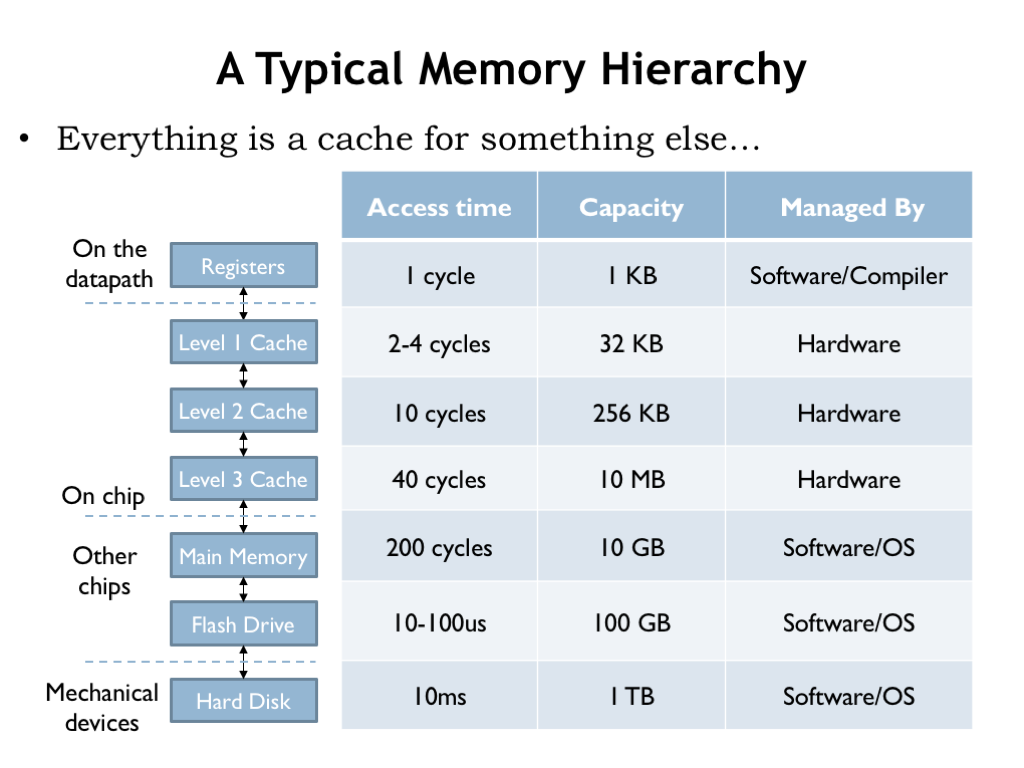
Here’s an example of a memory hierarchy that might be found on a modern computer. There are three levels of on-chip SRAM caches, followed by DRAM main memory and a flash-memory cache for the hard disk drive. The compiler is responsible for deciding which data values are kept in the CPU registers and which values require the use of LDs and STs. The 3-level cache and accesses to DRAM are managed by circuity in the memory system. After that the access times are long enough (many hundreds of instruction times) that the job of managing the movement of data between the lower levels of the hierarchy is turned over to software.
Whether managed by hardware or software, each layer of the memory system is designed to provide lower-latency access to frequently-accessed locations in the next, slower layer. But, as we’ll see, the implementation strategies will be quite different in the slower layers of the hierarchy.
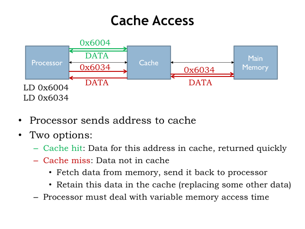
The processor starts an access by sending an address to the cache. If data for the requested address is held in the cache, it’s quickly returned to the CPU.
If the data we request is not in the cache, we have a cache miss, so the cache has to make a request to main memory to get the data, which it then returns to processor. Typically the cache will remember the newly fetched data, possibly replacing some older data in the cache.
Suppose a cache access takes 4 ns and a main memory access takes 40 ns. Then an access that hits in the cache has a latency of 4 ns, but an access that misses in the cache has a latency of 44 ns. The processor has to deal with the variable memory access time, perhaps by simply waiting for the access to complete, or, in modern hyper-threaded processors, it might execute an instruction or two from another programming thread.
Basic Cache Algorithm
Here’s a start at building a cache. The cache will hold many different blocks of data; for now let’s assume each block is an individual memory location. Each data block is tagged with its address. A combination of a data block and its associated address tag is called a cache line.
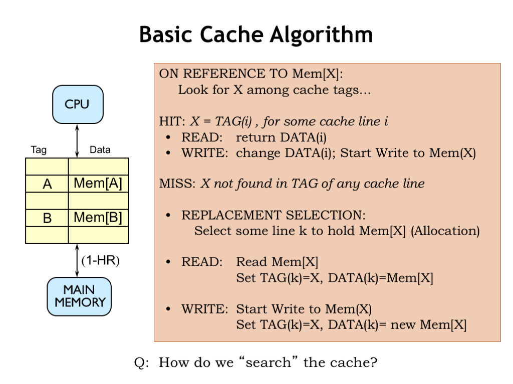
When an address is received from the CPU, we’ll search the cache looking for a block with a matching address tag. If we find a matching address tag, we have a cache hit. On a read access, we’ll return the data from the matching cache line. On a write access, we’ll update the data stored in the cache line and, at some point, update the corresponding location in main memory.
If no matching tag is found, we have a cache miss. So we’ll have to choose a cache line to use to hold the requested data, which means that some previously cached location will no longer be found in the cache. For a read operation, we’ll fetch the requested data from main memory, add it to the cache (updating the tag and data fields of the cache line) and, of course, return the data to the CPU. On a write, we’ll update the tag and data in the selected cache line and, at some point, update the corresponding location in main memory.
So the contents of the cache are determined by the memory requests made by the CPU. If the CPU requests a recently-used address, chances are good the data will still be in the cache from the previous access to the same location. As the working set slowly changes, the cache contents will be updated as needed. If the entire working set can fit into the cache, most of the requests will be hits and the AMAT will be close to the cache access time. So far, so good!
Of course, we’ll need to figure how to quickly search the cache, i.e., we’ll a need fast way to answer the question of whether a particular address tag can be found in some cache line. That’s our next topic.
Direct-Mapped Caches
The simplest cache hardware consists of an SRAM with a few additional pieces of logic. The cache hardware is designed so that each memory location in the CPU’s address space maps to a particular cache line, hence the name direct-mapped (DM) cache. There are, of course, many more memory locations then there are cache lines, so many addresses are mapped to the same cache line and the cache will only be able to hold the data for one of those addresses at a time.
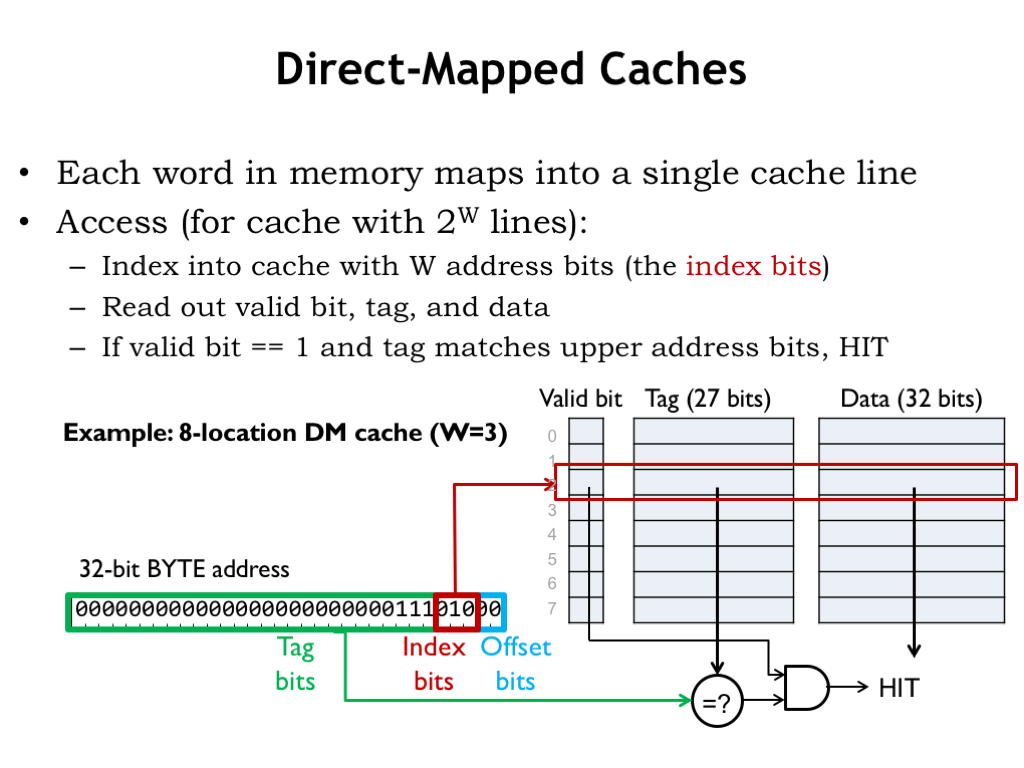
The operation of a DM cache is straightforward. We’ll use part of the incoming address as an index to select a single cache line to be searched. The search consists of comparing the rest of the incoming address with the address tag of the selected cache line. If the tag matches the address, there’s a cache hit and we can immediately use the data in the cache to satisfy the request.
In this design, we’ve included an additional valid bit which is 1 when the tag and data fields hold valid information. The valid bit for each cache line is initialized to 0 when the cache is powered on, indicating that all cache lines are empty. As data is brought into the cache, the valid bit is set to 1 when the cache line’s tag and data fields are filled. The CPU can request that the valid bit be cleared for a particular cache line — this is called flushing the cache. If, for example, the CPU initiates a read from disk, the disk hardware will read its data into a block of main memory, so any cached values for that block will be out-of-date. So the CPU will flush those locations from the cache by marking any matching cache lines as invalid.
Let’s see how this works using a small DM cache with 8 lines where each cache line contains a single word (4 bytes) of data. Here’s a CPU request for the location at byte address 0xE8. Since there 4 bytes of data in each cache line, the bottom 2 address bits indicate the appropriate byte offset into the cached word. Since the cache deals only with word accesses, the byte offset bits aren’t used.
Next, we’ll need to use 3 address bits to select which of the 8 cache lines to search. We choose these cache index bits from the low-order bits of the address. Why? Well, it’s because of locality. The principle of locality tells us that it’s likely that the CPU will be requesting nearby addresses and for the cache to perform well, we’d like to arrange for nearby locations to be able to be held in the cache at the same time. This means that nearby locations will have to be mapped to different cache lines. The addresses of nearby locations differ in their low-order address bits, so we’ll use those bits as the cache index bits — that way nearby locations will map to different cache lines.
The data, tag and valid bits selected by the cache line index are read from the SRAM. To complete the search, we check the remaining address against the tag field of the cache. If they’re equal and the valid bit is 1, we have a cache hit, and the data field can be used to satisfy the request.
How come the tag field isn’t 32 bits, since we have a 32-bit address? We could have done that, but since all values stored in cache line 2 will have the same index bits (0b010), we saved a few bits of SRAM and chose not save those bits in the tag. In other words, there’s no point in using SRAM to save bits we can generate from the incoming address.
So the cache hardware in this example is an 8-location by 60 bit SRAM plus a 27-bit comparator and a single AND gate. The cache access time is the access time of the SRAM plus the propagation delays of the comparator and AND gate. About as simple and fast as we could hope for.
The downside of the simplicity is that for each CPU request, we’re only looking in a single cache location to see if the cache holds the desired data. Not much of search is it? But the mapping of addresses to cache lines helps us out here. Using the low-order address bit as the cache index, we’ve arranged for nearby locations to be mapped to different cache lines. So, for example, if the CPU were executing an 8-instruction loop, all 8 instructions can be held in the cache at the same time. A more complicated search mechanism couldn’t improve on that. The bottom line: this extremely simple search is sufficient to get good cache hit ratios for the cases we care about.
Conflict Misses
DM caches do have an Achilles heel. Consider running the 3-instruction LOOPA code with the instructions located starting at word address 1024 and the data starting at word address 37 where the program is making alternating accesses to instruction and data, e.g., a loop of LD instructions.
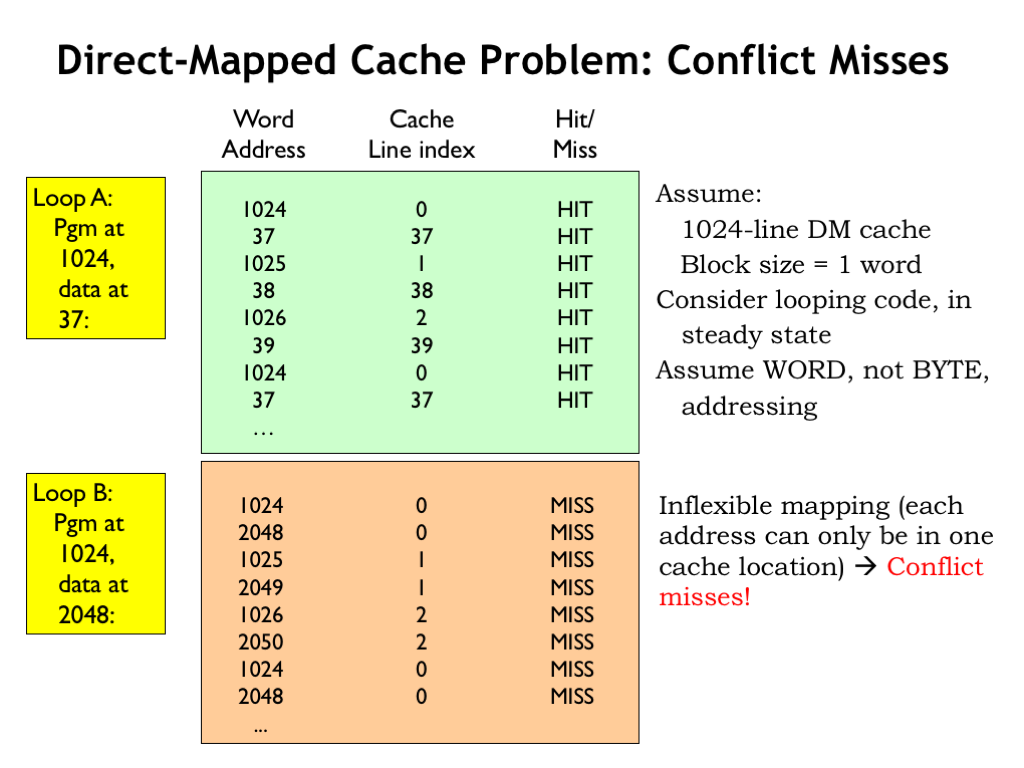
Assuming a 1024-line DM cache with a block size of 1, the steady state hit ratio will be 100% once all six locations have been loaded into the cache since each location is mapped to a different cache line.
Now consider the execution of the same program, but this time the data has been relocated to start at word address 2048. Now the instructions and data are competing for use of the same cache lines. For example, the first instruction (at address 1024) and the first data word (at address 2048) both map to cache line 0, so only one them can be in the cache at a time. So fetching the first instruction fills cache line 0 with the contents of location 1024, but then the first data access misses and then refills cache line 0 with the contents of location 2048. The data address is said to conflict with the instruction address. The next time through the loop, the first instruction will no longer be in the cache and its fetch will cause a cache miss, called a conflict miss. So in the steady state, the cache will never contain the word requested by the CPU.
This is very unfortunate! We were hoping to design a memory system that offered the simple abstraction of a flat, uniform address space. But in this example we see that simply changing a few addresses results in the cache hit ratio dropping from 100% to 0%. The programmer will certainly notice her program running 10 times slower!
So while we like the simplicity of DM caches, we’ll need to make some architectural changes to avoid the performance problems caused by conflict misses.
Associative Caches
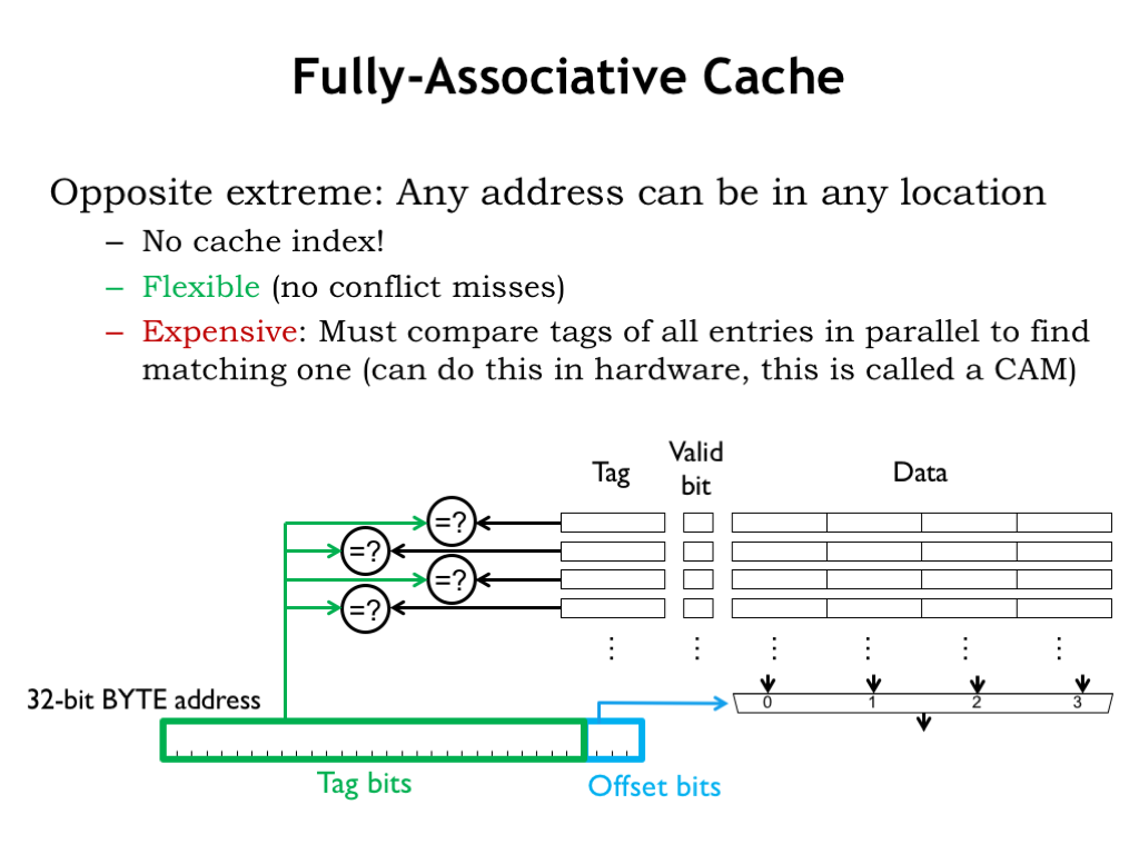
A fully-associative (FA) cache has a tag comparator for each cache line. So the tag field of every cache line in a FA cache is compared with the tag field of the incoming address. Since all cache lines are searched, a particular memory location can be held in any cache line, which eliminates the problems of address conflicts causing conflict misses. The cache shown here can hold 4 different 4-word blocks, regardless of their address. The example from the end of the previous segment required a cache that could hold two 3-word blocks, one for the instructions in the loop, and one for the data words. This FA cache would use two of its cache lines to perform that task and achieve a 100% hit ratio regardless of the addresses of the instruction and data blocks.
FA caches are very flexible and have high hit ratios for most applications. Their only downside is cost: the inclusion of a tag comparator for each cache line to implement the parallel search for a tag match adds substantially the amount of circuitry required when there are many cache lines. Even the use of hybrid storage/comparison circuitry, called a content-addressable memory, doesn’t make a big dent in the overall cost of a FA cache.
DM caches searched only a single cache line. FA caches search all cache lines. Is there a happy middle ground where some small number of cache lines are searched in parallel?
Replacement Policies
There’s one final issue to resolve associative caches. When there’s a cache miss, which cache line should be chosen to hold the data that will be fetched from main memory? That’s not an issue with DM caches, since each data block can only be held in one particular cache line, determined by its address. But in N-way SA caches, there are N possible cache lines to choose from, one in each of the ways. And in a FA cache, any of the cache lines can be chosen.
So, how to choose? Our goal is to choose to replace the contents of the cache line which will minimize the impact on the hit ratio in the future.
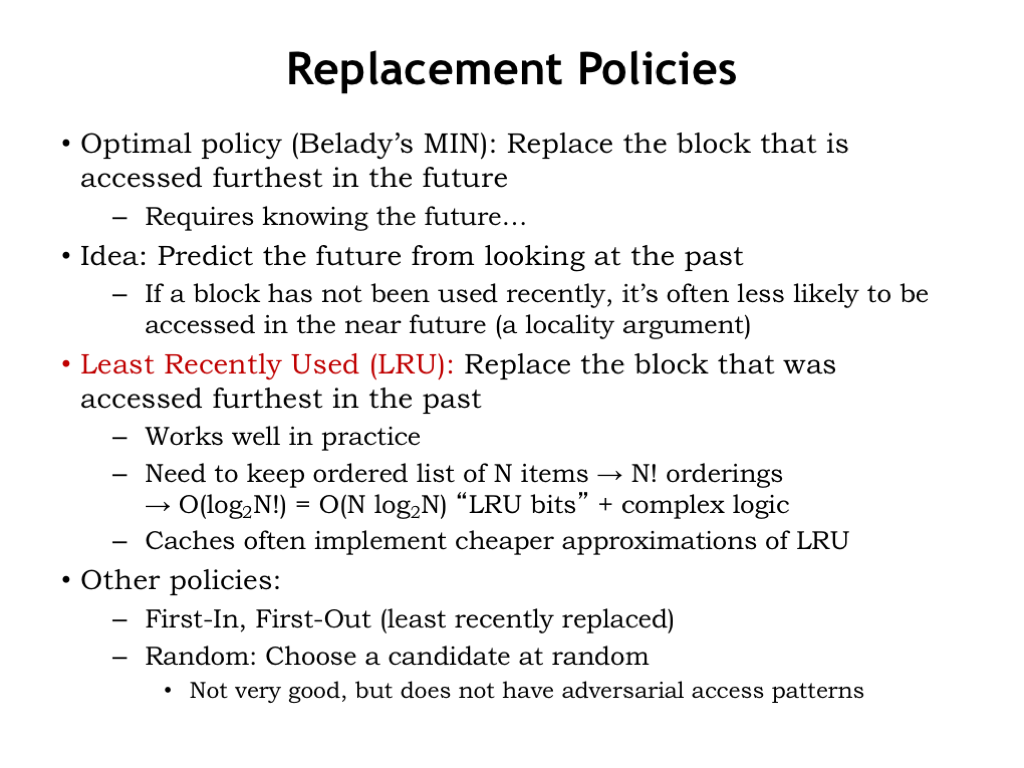
The optimal choice is to replace the block that is accessed furthest in the future (or perhaps is never accessed again). But that requires knowing the future…
Here’s an idea: let’s predict future accesses by looking at recent accesses and applying the principle of locality. If a block has not been recently accessed, it’s less likely to be accessed in the near future.
That suggests the least-recently-used replacement strategy, usually referred to as LRU: replace the block that was accessed furthest in the past. LRU works well in practice, but requires us to keep a list ordered by last use for each set of cache lines, which would need to be updated on each cache access. When we needed to choose which member of a set to replace, we’d choose the last cache line on this list. For an 8-way SA cache there are 8! possible orderings, so we’d need log2(8!) = 16 state bits to encode the current ordering. The logic to update these state bits on each access isn’t cheap; basically you need a lookup table to map the current 16-bit value to the next 16-bit value. So most caches implement an approximation to LRU where the update function is much simpler to compute.
There are other possible replacement policies: First-in, first-out, where the oldest cache line is replaced regardless of when it was last accessed. And Random, where some sort of pseudo-random number generator is used to select the replacement.
All replacement strategies except for random can be defeated. If you know a cache’s replacement strategy you can design a program that will have an abysmal hit rate by accessing addresses you know the cache just replaced. I’m not sure I care about how well a program designed to get bad performance runs on my system, but the point is that most replacement strategies will occasionally cause a particular program to execute much more slowly than expected.
When all is said and done, an LRU replacement strategy or a close approximation is a reasonable choice.
Write Strategies
Okay, one more cache design decision to make, then we’re done!
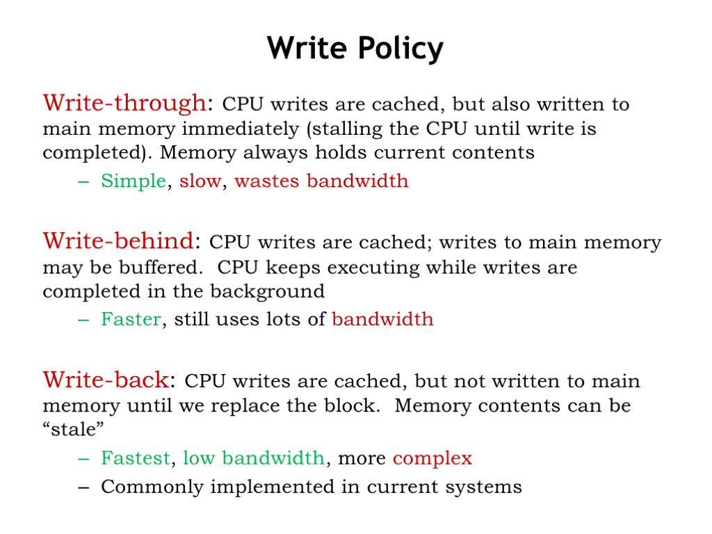
How should we handle memory writes in the cache? Ultimately we’ll need update main memory with the new data, but when should that happen?
The most obvious choice is to perform the write immediately. In other words, whenever the CPU sends a write request to the cache, the cache then performs the same write to main memory. This is called write-through. That way main memory always has the most up-to-date value for all locations. But this can be slow if the CPU has to wait for a DRAM write access — writes could become a real bottleneck! And what if the program is constantly writing a particular memory location, e.g., updating the value of a local variable in the current stack frame? In the end we only need to write the last value to main memory. Writing all the earlier values is waste of memory bandwidth.
Suppose we let the CPU continue execution while the cache waits for the write to main memory to complete — this is called write-behind. This will overlap execution of the program with the slow writes to main memory. Of course, if there’s another cache miss while the write is still pending, everything will have to wait at that point until both the write and subsequent refill read finish, since the CPU can’t proceed until the cache miss is resolved.
The best strategy is called write-back where the contents of the cache are updated and the CPU continues execution immediately. The updated cache value is only written to main memory when the cache line is chosen as the replacement line for a cache miss. This strategy minimizes the number of accesses to main memory, preserving the memory bandwidth for other operations. This is the strategy used by most modern processors.
Conclusion
That concludes our discussion of caches, which was motivated by our desire to minimize the average memory access time by building a hierarchical memory system that had both low latency and high capacity.
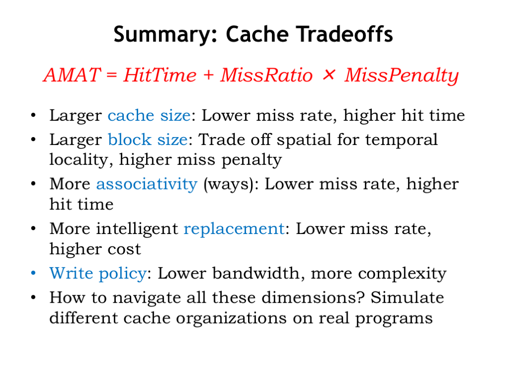
There were a number of strategies we employed to achieve our goal.
Increasing the number of cache lines decreases AMAT by decreasing the miss ratio.
Increasing the block size of the cache let us take advantage of the fast column accesses in a DRAM to efficiently load a whole block of data on a cache miss. The expectation was that this would improve AMAT by increasing the number of hits in the future as accesses were made to nearby locations.
Increasing the number of ways in the cache reduced the possibility of cache line conflicts, lowering the miss ratio.
Choosing the least-recently used cache line for replacement minimized the impact of replacement on the hit ratio.
And, finally, we chose to handle writes using a write-back strategy with dirty bits.
How do we make the tradeoffs among all these architectural choices? As usual, we simulate different cache organizations and chose the architectural mix that provides the best performance on our benchmark programs.
Assignment 5: Exploring Memory Hierarchy and Cache Utilization
In this activity, you may work in pairs or individually. You may not use ChatGPT or similar tools in any way, shape, or form on this activity. If there is any indication that one of those tools was used, you will received an automatic zero. Instead, working with your peer to do your best answering the questions throughout. Many of the questions are are open-ended, and thus have many possible answers, so I would expect them to vary widely between submissions.
Instructions
You will answer each of the below questions and submit them via the online assignment in Gradescope. I encourage you to spend some time thinking through these questions, working them out of paper (making notes and drawing pictures, where necessary). Then, after you feel good about your answer, enter them into Gradescope.
Model 1: Caches
Imagine you're an aspiring chef collecting recipes and cooking utensils as you progress in your culinary journey. You can store your culinary items in three places: your kitchen, your pantry, and the grocery store.
- When you are in cooking right now, which place is the most convenient? Where is the least convenient?
- Which place can hold the most ingredients and utensils?
- When you leave your kitchen to serve food elsewhere, how do you pick what items to bring with you?
- How might you change your utensils and ingredients with you in the kitchen when you are cooking a new recipe?
Model 2: Lookup
When a program tries to access memory, before the request goes onto the bus, it is passed through one or more caches. Each cache must quickly answer the question: does it have the data?
-
If the array below starts at (32-bit) address
0x00 00 FF 00, what is the address of the last element?int array[20]; -
Considering the four bytes of a 32-bit address, which address byte relates most to spatial locality?
-
A cache is very similar to a hash table. As we have learned, we want hash values to be across a large range. Caches use a very simple hashing algorithm of selecting a subset of the address bits. Discuss which range(s) you might use.
-
(advanced) Which part of the address often indicates whether the access is to the stack, heap, or global variables?
Unlike a hash table, caches do not resize, rehash, or otherwise move elements. Caches chain elements to a limited extent if they hash to the same location in the cache.
Model 3: Hardware
We can describe a cache using three numbers: $S$, $E$, and $B$. Let's break down what each of these parameters represents and how the first two relate to cache organization:
-
$S$ (Set count): This represents the number of sets in the cache. A set is a collection of cache lines where any new block from memory can be placed. The cache is divided into $S$ sets to allow for more efficient data storage and retrieval. The way a block is mapped to a specific set can vary based on the cache's mapping strategy (direct-mapped, fully associative, or set-associative).
-
$E$ (Number of cache lines per set): This represents the number of cache lines (or blocks) in each set. If $E = 1$, the cache is direct-mapped, meaning each set contains only one cache line. If $E$ is equal to the total number of cache lines, the cache is fully associative, meaning a block can be placed in any cache line. If $E$ is between 1 and the total number of cache lines, the cache is set-associative, meaning each set contains $E$ cache lines, and a block can be placed in any of the lines within a given set.
-
$B$ (Block size): This represents the size of each cache block (or line) in bytes. Each block is a unit of data transferred between the cache and main memory, and $B$ determines how much data is moved and stored in each cache operation.
These parameters ($S$, $E$, and $B$) together define the cache's size, structure, and behavior, impacting its performance, efficiency, and cost. Understanding how $S$ and $E$ relate helps in designing and analyzing cache systems, balancing trade-offs between speed, size, and cost.
The following figure shows how the first two relate to the cache organization.
-
The hashing bits from the previous model are actually the set index bits. If there are $S$ sets, how many bits are required for this purpose?
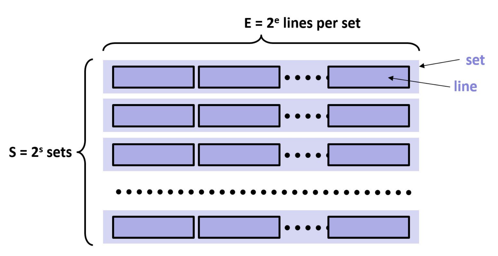
-
Cache lines contain blocks of data. The spatial locality bits are the block offset, which select the byte(s) from the block to return. How many bits are required for this purpose?
-
On selecting a cache set using the index bits, the cache must search (simultaneously as this is hardware) all of its lines to see whether any match the address. Each check is done using the remaining bits of the address. These bits are the tag. If $m$ is the number of address bits, how many bits are in the tag ($t$)?
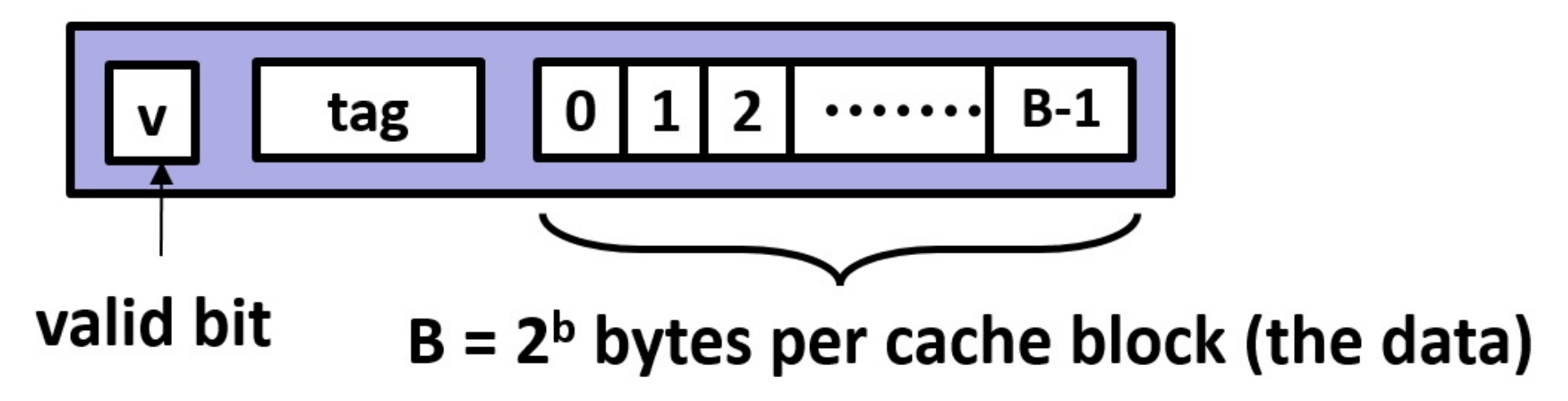
Cache lines also contain a valid bit to store whether this line is valid. Sets in caches will have one or more lines. If there is only one line, that cache is termed ‘direct mapped’. If there is only one set, then the cache is termed ‘fully associative’. Otherwise, the cache is considered E-way associative.
- Associativity has trade-offs. Remember that hardware costs space and energy. Between direct mapped and fully
associative, select the one that:
- Requires the most hardware
- Can determine whether a cache line is present fastest
- Is more likely to have the data present
- There are three basic types of cache misses. We also rate caches for their miss rates, which are misses/accesses. When an address is read for the very first time, where is it?
- The program accesses
array[0],array[1],array[2], andarray[3](see Model 2). At minimum, how large should $B$ be for there to be (ideally) only 1 miss?
Model 4: Replacement
Although not all college students do this (take for example one of my roommates!), let’s consider hanging your shirts in a closet. Imagine that your closet has limited space, but that you also have a box under your bed to store additional clothes.
- Your closet is full and you have received a new shirt. How do you make room in your closet for
this shirt?
- Pick randomly
- Box up the newest shirt
- Box up your oldest shirt
- Box up a shirt you haven’t worn in a while
- I use a different policy to replace my shirts (seasonal, etc)
- For the previous question, what additional information would you need to:
- Make the decision
- Determine whether the decision is best
When a cache access misses, the new address and its associated line is added to the appropriate set. Caches do not “rehash” addresses on a collision, instead the cache must select a line to replace in that set. Similarly, every cache line also maintains additional data in order to determine which cache line to replace.
- Caches seek to exploit temporal and spatial locality to mitigate the memory wall (i.e., the vast latency difference between a CPU cycle and a memory access). Consider the following access stream going to a set, where $E = 2$. Using the common least recently used (LRU) replacement policy, mark which accesses will hit and which will miss: $A$, $B$, $A$, $C$, $B$, $C$, $A$
- Could a different replacement algorithm have done better? If so, how?
- When a cache line is replaced, it is termed evicted. What should the cache do with the evicted line?
Model 5: Writing to Cache Lines
-
When a processor writes to a memory location, from where does the data come?
-
When a processor writes to a cache line present, the access hits in the cache. However, there is the question of what to do with the written data. Should the cache immediately update memory? Is there locality in the writes? How did we handle this code before?
for (int i = 1; i < (1000 * 1000); i++)
    a[0] += a[i];
If the cache caches the written values, then the cache is write back (WB). If it immediately updates memory, then it is write through (WT).
- In a write back cache, what must the cache do in when a cache line is evicted? Does the cache line need additional information?
- Now imagine writing to a location that is not already in cache. Do you think the cache should allocate a cache line to store the new data, or should the write skip the cache and go directly to memory? Why or why not?
The choice described in the previous question is termed write allocate (WA) vs. write no allocate (WNA). However, most architectures make both write design choices together, with the common pairings being WBWA and WTWNA.
- (advanced) When might it be advantageous to use each of these?
Note: This activity is based on one from Carnegie Mellon University (https://www.cs.cmu.edu/afs/cs/academic/class/15213-m19/www/activities/213_lecture12.pdf).
Assessment Rubric
Model 1: Caches (2 points)
- Identification of Convenience and Capacity: Were the most and least convenient storage locations identified appropriately? Was the place with the most storage capacity correctly identified?
- Consideration of Selection Process: Did the student provide a logical process for selecting items to bring when leaving the kitchen?
Model 2: Lookup (5 points)
- Understanding of Addressing: Was the address of the last element correctly determined? Was the significance of spatial locality addressed?
- Discussion of Cache Hashing: Was there a meaningful discussion about cache hashing algorithms and address ranges?
- Identification of Address Part Significance: Was there an understanding of the significance of different address parts regarding memory access types?
- Comprehension of Cache Misses: Was there a clear understanding of where a newly accessed address resides initially?
Model 3: Hardware (5 points)
- Understanding of Address Bits: Were the calculations for required address bits for set index, block offset, and tag correct?
- Appreciation of Cache Associativity: Was there a clear understanding of the trade-offs between different cache associativity levels?
- Consideration of Miss Rates: Was the understanding of cache miss rates and their implications demonstrated effectively?
Model 4: Replacement (5 points)
- Application of Closet Metaphor: Did the student effectively apply the closet metaphor to cache line replacement policies?
- Justification of Replacement Strategies: Was there a logical rationale provided for selecting a particular replacement strategy?
Model 5: Writing to Cache Lines (5 points)
- Understanding of Write Policies: Was there a clear understanding of write-back and write-through cache policies?
- Consideration of Cache Allocation Choices: Did the student discuss the advantages and disadvantages of write allocate and write no allocate approaches?
- Insight into Write Handling: Was there insight into the handling of writes in cache lines and their eviction?
Overall Presentation (5 points)
- Accuracy: Are the responses accurate and well-supported?
- Clarity and Organization: Were the responses clear, organized, and easy to follow?
- Depth of Analysis: Did the student delve into the topics with sufficient depth and insight?
- Grammar and Style: Were the responses well-written with proper grammar and style?
Submitting Your Work
Your work must be submitted to Anchor for degree credit and to Gradescope for grading.
- Complete the work in Gradescope by navigating tot he appropriate link.
- Export it as a pdf using th Google Chrome plugin: https://gofullpage.com/. This plugin will do multiple screen captures while scrolling through your document, and then stitch them into a pdf that you can download.
- Upload the generated pdf to Anchor using the form below.
Week 8 Participation
During the live class session this week, you will be asked to complete some of the problems that we went through in this material.
Your completion of these questions and answers, and your engagement during the live class will make up your Weekly Participation Score.
Process Execution
Welcome to week 9 of Computer Systems! This week we will move up an additional layer and focus on operating system concerns, particularly around how the computer managed running multiple processes and switching between them during normal operation. We will also touch on a few command-line tools in Linux/Unix systems that we commonly use to manage and monitor OS processes.
Topics Covered
- Exceptions
- User & Kernel Modes
- Context Switches
- Process Control & Multiprocessing
- Process Management Tools (
metrics,top,ps)
Learning Outcomes
After this week, you will be able to:
- Understand the role of exceptions in operating systems and how they handle unexpected events and interrupts.
- Differentiate between user mode and kernel mode, and comprehend the privilege levels associated with each mode.
- Explain the concept of context switches and their significance in multitasking environments, including the steps involved and strategies to reduce overhead.
- Describe the process control and multiprocessing mechanisms in operating systems, including process creation, scheduling, and termination.
- Demonstrate proficiency in using process management tools (e.g., 'top' and 'ps') to monitor system resources and analyze process performance.
Materials in this module are based on or taken from the below source: Operating Systems and Middleware: Supporting Controlled Interaction by Max Hailperin is licensed under a Creative Commons Attribution-ShareAlike 3.0 Unported License.
An Operating System "process"
Processes play a central role in the view of an operating system as experienced by most system administrators, application programmers, and other moderately sophisticated computer users. In particular, the technical concept of process comes the closest to the informal idea of a running program.
The concept of process is not entirely standardized across different operating systems. Not only do some systems use a different word (such as "task"), but also the details of the definition vary. Nonetheless, most mainstream systems are based on definitions that include the following:
-
One or more threads: Because a process embodies a running program, often the process will be closely associated with a single thread. However, some programs are designed to divide work among multiple threads, even if the program is run only once. (For example, a web browser might use one thread to download a web page while another thread continues to respond to the user interface.)
In operating systems, a thread is the smallest sequence of programmed instructions that can be managed independently by a scheduler. Threads enable parallel execution of tasks within a single process, improving the efficiency of resource usage and application performance. We will discuss threads in more detail shortly.
-
Memory accessible to those threads: The word "accessible" implies that some sort of protection scheme ensures that the threads within a process access only the memory for which that process has legitimate access rights. As you will see, the mainstream protection approach is for each process to have its own virtual memory address space, shared by the threads within that process. However, I will also present an alternative, in which all processes share a single address space, but with varying access rights to individual objects within that address space. In any case, the access rights are assigned to the process, not to the individual threads.
-
Other access rights: A process may also hold the rights to resources other than memory. For example, it may have the right to update a particular file on disk or to service requests arriving over a particular network communication channel. We will sketch two general approaches by which a process can hold access rights. Either the process can hold a specific capability, such as the capability to write a particular file, or it can hold a general credential, such as the identification of the user for whom the process is running. In the latter case, the credential indirectly implies access rights, by way of a separate mechanism, such as access control lists.
-
Resource allocation context: Limited resources (such as space in memory or on disk) are generally associated with a process for two reasons. First, the process's termination may serve to implicitly release some of the resources it is holding, so that they may be reallocated. Operating systems generally handle memory in this way. Second, the process may be associated with a limited resource quota or with a billing account for resource consumption charges. For simplicity, I will not comment on these issues any further.
-
Miscellaneous context: Operating systems often associate other aspects of a running program's state with the process. For example, systems such as Linux and UNIX (conforming to the POSIX standard) keep track of each process's current working directory. That is, when any thread in the process accesses a file by name without explicitly indicating the directory containing the file, the operating system looks for the file starting from the process's current working directory. For historical reasons, the operating system tracks a single current working directory per process, rather than one per thread.
From this list, you can see that many of the key aspects of processes concern protection, and these are the aspects on which we will focus. But first, we will devote the next section to the basics of how the POSIX process management API can be used, such as how a thread running in one process creates another process and how a process exits. This section should serve to make the use of processes more concrete. Studying this API will also allow you to understand how the shell (command interpreter) executes user commands.
POSIX Process Management
All operating systems provide mechanisms for creating new processes, terminating existing processes, and performing related actions. The details vary from system to system. To provide a concrete example, I will present relevant features of the POSIX API, which is used by Linux and UNIX, including by Mac OS X.
In the POSIX approach, each process is identified by a process ID number, which is a positive integer. Each process
(with one exception) comes into existence through the forking of a parent process. The exception is the first
process created when the operating system starts running. A process forks off a new process whenever one of the threads
running in the parent process calls the fork procedure. In the parent process, the call to fork returns the process
ID number of the new child process. (If an error occurs, the procedure instead returns a negative number.) The process
ID number may be important to the parent later, if it wants to exert some control over the child or find out when the
child terminates.
Meanwhile, the child process can start running. The child process is in many regards a copy of the parent process. For protection purposes, it has the same credentials as the parent and the same capabilities for such purposes as access to files that have been opened for reading or writing. In addition, the child contains a copy of the parent's address space. That is, it has available to it all the same executable program code as the parent, and all of the same variables, which initially have the same values as in the parent. However, because the address space is copied instead of shared, the variables will start having different values in the two processes as soon as either performs any instructions that store into memory. (Special facilities do exist for sharing some memory; I am speaking here of the normal case.)
Because the child process is nearly identical to the parent, it starts off by performing the same action as the parent;
the fork procedure returns to whatever code called it. However, application programmers generally don't want the child
to continue executing all the same steps as the parent; there wouldn't be much point in having two processes if they
behaved identically. Therefore, the fork procedure gives the child process an indication that it is the child so that
it can behave differently. Namely, fork returns a value of 0 in the child. This contrasts with the return value in the
parent process, which is the child's process ID number, as mentioned earlier.
The normal programming pattern is for any fork operation to be immediately followed by an if statement that checks
the return value from fork. That way, the same program code can wind up following two different courses of action, one
in the parent and one in the child, and can also handle the possibility of failure, which is signaled by a negative
return value. The C program below shows an example of this; the parent and child processes are similar (both loop five
times, printing five messages at one-second intervals), but they are different enough to print different messages, as
shown in the sample output. Keep in mind that this output is only one possibility; not only can the ID number be
different, but the interleaving of output from the parent and child can also vary from run to run.
#include <unistd.h>
#include <stdio.h>

int main() {
    int loopCount = 5; // each process will get its own loopCount
    printf("I am still only one process.\n");
    pid_t returnedValue = fork();
    if (returnedValue < 0){
        // still only one process
        perror("error forking"); // report the error
        return -1;
    } else if (returnedValue == 0){
        // this must be the child process
            while(loopCount > 0) {
            printf("I am the child process.\n");
            loopCount--; // decrement child’s counter only
            sleep(1); // wait a second before repeating
            }
    }
    else {
        // this must be the parent process
        while (loopCount > 0){
            printf("I am the parent process; my child’s ID is %i\n", returnedValue);
            loopCount--; // decrement parent’s counter only
            sleep(1);
        }
    }
    return 0;
}
I am still only one process.
I am the child process.
I am the parent process; my child's ID is 23307
I am the parent process; my child's ID is 23307
I am the child process.
I am the parent process; my child's ID is 23307
I am the child process.
I am the parent process; my child's ID is 23307
I am the child process.
I am the parent process; my child's ID is 23307
I am the child process.
This example program also illustrates that the processes each get their own copy of the loopCount variable. Both start
with the initial value, 5, which was established before the fork. However, when each process decrements the counter,
only its own copy is affected.
In early versions of UNIX, only one thread ever ran in each process. As such, programs that involved concurrency needed
to create multiple processes using fork. In situations such as that, it would be normal to see a program like the one
above, which includes the full code for both parent and child. Today, however, concurrency within a program is normally
done using a multithreaded process. This leaves only the other big use of fork: creating a child process to run an
entirely different program. In this case, the child code in the forking program is only long enough to load in the new
program and start it running. This happens, for example, every time you type a program's name at a shell prompt; the
shell forks off a child process in which it runs the program. Although the program execution is distinct from the
process forking, the two are used in combination. Therefore, I will turn next to how a thread running in a process can
load a new program and start that program running.
The POSIX standard includes six different procedures, any one of which can be used to load in a new program and start it
running. The six are all variants on a theme; because they have names starting with exec, they are commonly called the
exec family. Each member of the exec family must be given enough information to find the new program stored in a file
and to provide the program with any arguments and environment variables it needs. The family members differ in exactly
how the calling program provides this information. Because the family members are so closely related, most systems
define only the execve procedure in the kernel of the operating system itself; the others are library procedures
written in terms of execve.
Because execl is one of the simpler members of the family, I will use it for an example. The program below prints out
a line identifying itself, including its own process ID number, which it gets using the getpid procedure. Then it uses
execl to run a program, named ps, which prints out information about running processes. After the call to execl
comes a line that prints out an error message, saying that the execution failed. You may find it surprising that the
error message seems to be issued unconditionally, without an if statement testing whether an error in fact occurred.
The reason for this surprising situation is that members of the exec family return only if an error occurs; if all is
well, the new program has started running, replacing the old program within the process, and so there is no possibility
of returning in the old program.
#include <unistd.h>
#include <stdio.h>

int main(){
    printf("This is the process with ID %i, before the exec.\n", getpid());
    execl("/bin/ps", "ps", "axl", NULL);
    perror("error execing ps");
    return -1;
}
Looking in more detail at the example program's use of execl, you can see that it takes several arguments that are
strings, followed by the special NULL pointer. The reason for the NULL is to mark the end of the list of strings;
although this example had three strings, other uses of execl might have fewer or more. The first string specifies
which file contains the program to run; here it is /bin/ps, that is, the ps program in the /bin directory, which
generally contains fundamental programs. The remaining strings are the so-called "command-line arguments," which are
made available to the program to control its behavior. Of these, the first is conventionally a repeat of the command's
name; here, that is ps. The remaining argument, axl, contains both the letters ax indicating that all processes
should be listed and the letter l indicating that more complete information should be listed for each process. As you
can see from the sample output below, the exact same process ID that is mentioned in the initial message shows up again
as the ID of the process running the ps axl command. The process ID remains the same because execl has changed what
program the process is running without changing the process itself.
This is the process with ID 3849, before the exec.
  UID   PID  ...  COMMAND
.
.
.
    0  3849  ...  ps axl
.
.
.
One inconvenience about execl is that to use it, you need to know the directory in which the program file is located.
For example, the previous program will not work if ps happens to be installed somewhere other than /bin on your
system. To avoid this problem, you can use execlp. You can give this variant a filename that does not include a
directory, and it will search through a list of directories looking for the file, just like the shell does when you type
in a command. This can be illustrated with an example program that combines fork with execlp:
#include <unistd.h>
#include <stdio.h>

int main() {
    pid_t returnedValue = fork();
    if (returnedValue < 0) {
        perror("error forking");
        return -1;
    }
    else if (returnedValue == 0) {
        execlp("xclock", "xclock", NULL);
        perror("error execing xclock");
        return -1;
    }
    else {
        return 0;
    }
}
This example program assumes you are running the X Window System, as on most Linux or UNIX systems. It runs xclock, a
program that displays a clock in a separate window. If you run the launcher program from a shell, you will see the
clock window appear, and your shell will prompt you for the next command to execute while the clock keeps running. This
is different than what happens if you type xclock directly to the shell. In that case, the shell waits for the xclock program to exit before prompting for another command. Instead, the example program is more similar to typing
xclock & to the shell. The & character tells the shell not to wait for the program to exit; the program is said to
run "in the background." The way the shell does this is exactly the same as the sample program: it forks off a child
process, executes the program in the child process, and allows the parent process to go on its way. In the shell, the
parent loops back around to prompt for another command.
When the shell is not given the & character, it still forks off a child process and runs the requested command in the
child process, but now the parent does not continue to execute concurrently. Instead the parent waits for the child
process to terminate before the parent continues. The same pattern of fork, execute, and wait would apply in any case
where the forking of a child process is not to enable concurrency, but rather to provide a separate process context in
which to run another program.
In order to wait for a child process, the parent process can invoke the waitpid procedure. This procedure takes three
arguments; the first is the process ID of the child for which the parent should wait, and the other two can be zero if
all you want the parent to do is to wait for termination. As an example of a process that waits for each of its child
processes, the program below shows a very stripped-down shell.
#include <unistd.h>
#include <stdio.h>
#include <sys/wait.h>
#include <stdlib.h>
#include <string.h>

int main() {
    char command[256]; // Array to hold the command

    while(1) { // Loop until return
        printf("Command (one word only)> ");
        fflush(stdout); // Make sure "Command" is printed immediately

        if (scanf("%255s", command) != 1) {
            fprintf(stderr, "Error reading command\n");
            return -1; // Exit if we fail to read a command
        }

        if (strcmp(command, "exit") == 0) {
            return 0; // Exit the loop if the command is "exit"
        } else {
            pid_t returnedValue = fork();
            if (returnedValue < 0) {
                perror("Error forking");
                return -1;
            } else if (returnedValue == 0) {
                execlp(command, command, NULL);
                perror(command); // If execlp returns, it must have failed
                return -1;
            } else {
                if (waitpid(returnedValue, NULL, 0) < 0) {
                    perror("Error waiting for child");
                    return -1;
                }
            }
        }
    }
}
This shell can be used to run the user's choice of commands, such as date, ls, and ps, as illustrated in the
output below. A real shell would allow command line arguments, offer background execution as an option, and provide many
other features. Nonetheless, you now understand the basics of how a shell runs programs
Command (one word only)> date
Thu Feb 12 09:33:26 CST 2024
Command (one word only)> ls
microshell microshell.c
Command (one word only)> ps
  PID TTY       TIME     CMD
23498 pts/2     00:00:00 bash
24848 pts/2     00:00:00 microshell
24851 pts/2     00:00:00 ps
Command (one word only)> exit
Notice that a child process might terminate prior to the parent process invoking waitpid. As such, the waitpid
procedure may not actually need to wait, contrary to what its name suggests. It may be able to immediately report the
child process's termination. Even in this case, invoking the procedure is still commonly referred to as "waiting for"
the child process. Whenever a child process terminates, if its parent is not already waiting for it, the operating
system retains information about the terminated process until the parent waits for it. A terminated process that has not
yet been waited for is known as a zombie. Waiting for a zombie makes its process ID number available for assignment to
a new process; the memory used to store information about the process can also be reused. This is known as the zombie.
At this point, you have seen many of the key elements of the process life cycle. Perhaps the most important omission is
that I haven't shown how processes can terminate, other than by returning from the main procedure. A process can
terminate itself by using the exit procedure (in Java, System.exit), or it can terminate another process using the
kill procedure (see the documentation for details).
Threads
Computer programs consist of instructions, and computers carry out sequences of computational steps specified by those instructions. We call each sequence of computational steps that are strung together one after another a thread. The simplest programs to write are single-threaded, with instructions that should be executed one after another in a single sequence. Programs can also have more than one thread of execution, each an independent sequence of computational steps, with few if any ordering constraints between the steps in one thread and those in another. Multiple threads can also come into existence by running multiple programs, or by running the same program more than once.
Note the distinction between a program and a thread: the program contains instructions, whereas the thread consists of the execution of those instructions. Even for single-threaded programs, this distinction matters. If a program contains a loop, then a very short program could give rise to a very long thread of execution. Also, running the same program ten times will give rise to ten threads, all executing one program.
Each thread has a lifetime, extending from the time its first instruction execution occurs until the time of its last instruction execution. If two threads have overlapping lifetimes, we say they are concurrent. One of the most fundamental goals of an operating system is to allow multiple threads to run concurrently on the same computer. That is, rather than waiting until the first thread has completed before a second thread can run, it should be possible to divide the computer’s attention between them. If the computer hardware includes multiple processors, then it will naturally be possible to run threads concurrently, one per processor. However, the operating system’s users will often want to run more concurrent threads than the hardware has processors. Therefore, the operating system will need to divide each processor’s attention between multiple threads.
In order to make the concept of concurrent threads concrete, we will next give an example of how to write a program that spawns multiple threads each time the program is run. Once you know how to create threads, we will explain some of the reasons why it is desirable to run multiple threads concurrently and will offer some typical examples of the uses to which threads are put.
Example of Multithreaded Programs
Whenever a program initially starts running, the computer carries out the program’s instructions in a single thread. Therefore, if the program is intended to run in multiple threads, the original thread needs at some point to spawn off a child thread that does some actions, while the parent thread continues to do others. (For more than two threads, the program can repeat the thread-creation step.) Most programming languages have an application programming interface (or API) for threads that includes a way to create a child thread. In this section, I will use the API for C that is called pthreads, for POSIX threads.
Realistic multithreaded programming requires the control of thread interactions. Therefore, my examples in this chapter are quite simple, just enough to show the spawning of threads.
To demonstrate the independence of the two threads, I will have both the parent and the child thread respond to a timer. One will sleep three seconds and then print out a message. The other will sleep five seconds and then print out a message. Because the threads execute concurrently, the second message will appear approximately two seconds after the first.
#include <pthread.h>
#include <unistd.h>
#include <stdio.h>

static void *child(void *ignored) {
    sleep(3);
    printf("Child is done sleeping 3 seconds.\n");
    return NULL;
}

int main(int argc, char *argv[]) {
    pthread_t child_thread;
    int code;
    code = pthread_create(&child_thread, NULL, child, NULL);
    if(code) {
        fprintf(stderr, "pthread_create failed with code %d\n", code);
    }
    sleep(5);
    printf("Parent is done sleeping 5 seconds.\n");
    return 0;
}
The above C program uses the pthreads API. The child procedure sleeps three seconds and prints a message. The main procedure creates a child_thread running the child procedure, and then itself sleeps five seconds and prints a message.
In addition to portable APIs, such as the Java and pthreads APIs, many systems provide their own non-portable APIs. For
example, Microsoft Windows has the Win32 API, with procedures such as CreateThread and Sleep.
Reasons for Using Concurrent Threads
You have now seen how a single execution of one program can result in more than one thread. Presumably, you were already at least somewhat familiar with generating multiple threads by running multiple programs, or by running the same program multiple times. Regardless of how the threads come into being, we are faced with a question. Why is it desirable for the computer to execute multiple threads concurrently, rather than waiting for one to finish before starting another? Fundamentally, most uses for concurrent threads serve one of two goals:
-
Responsiveness: allowing the computer system to respond quickly to something external to the system, such as a human user or another computer system. Even if one thread is in the midst of a long computation, another thread can respond to the external agent. Our example program illustrated responsiveness: both the parent and the child thread responded to a timer.
-
Resource utilization: keeping most of the hardware resources busy most of the time. If one thread has no need for a particular piece of hardware, another may be able to make productive use of it.
Each of these two general themes has many variations, some of which we explore in the remainder of this section. A third reason why programmers sometimes use concurrent threads is as a tool for modularization. With this, a complex system may be decomposed into a group of interacting threads.
Responsiveness
Let’s start by considering the responsiveness of a web server, which provides many client computers with the specific web pages they request over the Internet. Whenever a client computer makes a network connection to the server, it sends a sequence of bytes that contain the name of the desired web page. Therefore, before the server program can respond, it needs to read in those bytes, typically using a loop that continues reading in bytes from the network connection until it sees the end of the request. Suppose one of the clients is connecting using a very slow network connection, perhaps via a dial-up modem. The server may read the first part of the request and then have to wait a considerable length of time before the rest of the request arrives over the network. What happens to other clients in the meantime? It would be unacceptable for a whole website to grind to a halt, unable to serve any clients, just waiting for one slow client to finish issuing its request. One way some web servers avoid this unacceptable situation is by using multiple threads, one for each client connection, so that even if one thread is waiting for data from one client, other threads can continue interacting with the other clients. This figure illustrates the unacceptable single-threaded web server and the more realistic multithreaded on
On the client side, a web browser may also illustrate the need for responsiveness. Suppose you start loading in a very large web page, which takes considerable time to download. Would you be happy if the computer froze up until the download finished? Probably not. You expect to be able to work on a spreadsheet in a different window, or scroll through the first part of the web page to read as much as has already downloaded, or at least click on the Stop button to give up on the time-consuming download. Each of these can be handled by having one thread tied up loading the web page over the network, while another thread is responsive to your actions at the keyboard and mouse.
Resource Utilization
Turning to the utilization of hardware resources, the most obvious scenario is when you have a dual-processor computer. In this case, if the system ran only one thread at a time, only half the processing capacity would ever be used. Even if the human user of the computer system doesn’t have more than one task to carry out, there may be useful housekeeping work to keep the second processor busy. For example, most operating systems, if asked to allocate memory for an application program’s use, will store all zeros into the memory first. Rather than holding up each memory allocation while the zeroing is done, the operating system can have a thread that proactively zeros out unused memory, so that when needed, it will be all ready. If this housekeeping work (zeroing of memory) were done on demand, it would slow down the system’s real work; by using a concurrent thread to utilize the available hardware more fully, the performance is improved. This example also illustrates that not all threads need to come from user programs. A thread can be part of the operating system itself, as in the example of the thread zeroing out unused memory.
Even in a single-processor system, resource utilization considerations may justify using concurrent threads. Remember that a computer system contains hardware resources, such as disk drives, other than the processor. Suppose you have two tasks to complete on your PC: you want to scan all the files on disk for viruses, and you want to do a complicated photo-realistic rendering of a three-dimensional scene including not only solid objects, but also shadows cast on partially transparent smoke clouds. From experience, you know that each of these will take about an hour. If you do one and then the other, it will take two hours. If instead you do the two concurrently—running the virus scanner in one window while you run the graphics rendering program in another window—you may be pleasantly surprised to find both jobs done in only an hour and a half.
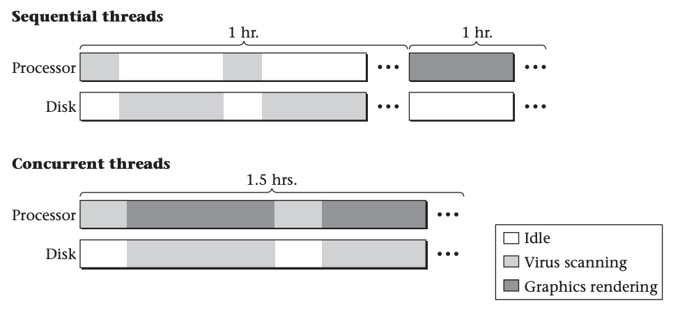
The explanation for the half-hour savings in elapsed time is that the virus scanning program spends most of its time using the disk drive to read files, with only modest bursts of processor activity each time the disk completes a read request, whereas the rendering program spends most of its time doing processing, with very little disk activity. As illustrated above, running them in sequence leaves one part of the computer’s hardware idle much of the time, whereas running the two concurrently keeps the processor and disk drive both busy, improving the overall system efficiency. Of course, this assumes the operating system’s scheduler is smart enough to let the virus scanner have the processor’s attention (briefly) whenever a disk request completes, rather than making it wait for the rendering program. This is known as scheduling, and is a topic that we won't get into in this course.
As you have now seen, threads can come from multiple sources and serve multiple roles. They can be internal portions of the operating system, as in the example of zeroing out memory, or part of the user’s application software. In the latter case, they can either be dividing up the work within a multithreaded process, such as the web server and web browser examples, or can come from multiple independent processes, as when a web browser runs in one window and a spreadsheet in another. Regardless of these variations, the typical reasons for running the threads concurrently remain unchanged: either to provide increased responsiveness or to improve system efficiency by more fully utilizing the hardware.
We just explored the application programmer’s view of threads: how and why the programmer would use concurrent threads. This sets us up for the next question: how does the operating system support the application programmer’s desire for concurrently executing threads? Stay tuned!
Context Switching
In order for the operating system to have more than one thread underway on a processor, the system needs to have some mechanism for switching attention between threads. In particular, there needs to be some way to leave off from in the middle of a thread’s sequence of instructions, work for a while on other threads, and then pick back up in the original thread right where it left off. In order to explain this context switching as simply as possible, I will initially assume that each thread is executing code that contains, every once in a while, explicit instructions to temporarily switch to another thread. Once you understand this mechanism, I can then build on it for the more realistic case where the thread contains no explicit thread-switching points, but rather is automatically interrupted for thread switches.
Thread switching is often called context switching, because it switches from the execution context of one thread to that of another thread. Many authors, however, use the phrase context switching differently, to refer to switching processes with their protection contexts. If the distinction matters, the clearest choice is to avoid the ambiguous term context switching and use the more specific thread switching or process switching
Example
Suppose we have two threads, A and B, and we use A1, A2, A3, and so forth as names for the instruction execution steps
that constitute A, and similarly for B. In this case, one possible execution sequence might be as shown below.
As I will explain subsequently, when thread A executes switchFromTo(A, B) the computer starts executing instructions from
thread B. In a more realistic example, there might be more than two threads, and each might run for many more steps
(both between switches and overall), with only occasionally a new thread starting or an existing thread exiting.
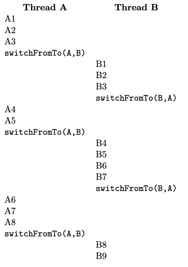
Our goal is that the steps of each thread form a coherent execution sequence. That is, from the perspective of thread A, its execution should not be much different from one in which A1 through A8 occurred consecutively, without interruption, and similarly for thread B’s steps B1 through B9. Suppose, for example, steps A1 and A2 load two values from memory into registers, A3 adds them, placing the sum in a register, and A4 doubles that register’s contents, so as to get twice the sum. In this case, we want to make sure that A4 really does double the sum computed by A1 through A3, rather than doubling some other value that thread B’s steps B1 through B3 happen to store in the same register. Thus, we can see that switching threads cannot simply be a matter of a jump instruction transferring control to the appropriate instruction in the other thread. At a minimum, we will also have to save registers into memory and restore them from there, so that when a thread resumes execution, its own values will be back in the registers.
Basic Case
In order to focus on the essentials, let’s put aside the issue of how threads start and exit. Instead, let’s focus just on the normal case where one thread in progress puts itself on hold and switches to another thread where that other thread last left off, such as the switch from A5 to B4 in the preceding example. To support switching threads, the operating system will need to keep information about each thread, such as at what point that thread should resume execution. If this information is stored in a block of memory for each thread, then we can use the addresses of those memory areas to refer to the threads. The block of memory containing information about a thread is called a thread control block or task control block (TCB). Thus, another way of saying that we use the addresses of these blocks is to say that we use pointers to thread control blocks to refer to threads.
Our fundamental thread-switching mechanism will be the switchFromTo procedure, which takes two of these thread control
block pointers as parameters: one specifying the thread that is being switched out of, and one specifying the next
thread, which is being switched into. In our running example, A and B are pointer variables pointing to the two threads’
control blocks, which we use alternately in the roles of outgoing thread and next thread. For example, the program for
thread A contains code after instruction A5 to switch from A to B, and the program for thread B contains code after
instruction B3 to switch from B to A. Of course, this assumes that each thread knows both its own identity and the
identity of the thread to switch to. Later, we will see how this unrealistic assumption can be eliminated. For now,
though, let’s see how we could write the switchFromTo procedure so that switchFromTo(A, B) would save the current
execution status information into the structure pointed to by A, read back previously saved information from the
structure pointed to by B, and resume where thread B left off.
We already saw that the execution status information to save includes not only a position in the program, often called the program counter (PC) or instruction pointer (IP), but also the contents of registers. Another critical part of the execution status for programs compiled with most higher level language compilers is a portion of the memory used to store a stack, along with a stack pointer register that indicates the position in memory of the current top of the stack.
When a thread resumes execution, it must find the stack the way it left it. For example, suppose thread A pushes two items on the stack and then is put on hold for a while, during which thread B executes. When thread A resumes execution, it should find the two items it pushed at the top of the stack—even if thread B did some pushing of its own and has not yet gotten around to popping. We can arrange for this by giving each thread its own stack, setting aside a separate portion of memory for each of them. When thread A is executing, the stack pointer (or SP register) will be pointing somewhere within thread A’s stack area, indicating how much of that area is occupied at that time. Upon switching to thread B, we need to save away A’s stack pointer, just like other registers, and load in thread B’s stack pointer. That way, while thread B is executing, the stack pointer will move up and down within B’s stack area, in accordance with B’s own pushes and pops.
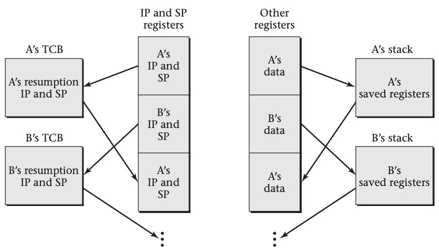
Having discovered this need to have separate stacks and switch stack pointers, we can simplify the saving of all other
registers by pushing them onto the stack before switching and popping them off the stack after switching, as shown in the figure above. We can use this approach to outline the code for switching from the outgoing thread to the next thread,
using outgoing and next as the two pointers to thread control blocks. (When switching from A to B, outgoing will be A
and next will be B. Later, when switching back from B to A, outgoing will be B and next will be A.) We will use
outgoing->SP and outgoing->IP to refer to two slots within the structure pointed to by outgoing, the slot used to save
the stack pointer and the one used to save the instruction pointer. With these assumptions, our code has the following
general form:
  push each register on the (outgoing thread’s) stack
  store the stack pointer into outgoing->SP
  load the stack pointer from next->SP
  store label L’s address into outgoing->IP
  load in next->IP and jump to that address
L:
  pop each register from the (resumed outgoing thread’s) stack
Note that the code before the label (L) is done at the time of switching away from the outgoing thread, whereas the code
after that label is done later, upon resuming execution when some other thread switches back to the original one.
This code not only stores the outgoing thread’s stack pointer away, but also restores the next thread’s stack pointer.
Later, the same code will be used to switch back. Therefore, we can count on the original thread’s stack pointer to have
been restored when control jumps to label L. Thus, when the registers are popped, they will be popped from the original
thread’s stack, matching the pushes at the beginning of the code.
Linux Example
We can see how this general pattern plays out in a real system, by looking at the thread-switching code from the Linux operating system for the x86 architecture.
This is real code extracted from an old version of the Linux kernel, though with some peripheral complications left
out. The stack pointer register is named %esp, and when this code starts running, the registers known as %ebx and %esi
contain the outgoing and next pointers, respectively. Each of those pointers is the address of a thread control block.
The location at offset 812 within the TCB contains the thread’s instruction pointer, and the location at offset 816
contains the thread’s stack pointer. (That is, these memory locations contain the instruction pointer and stack pointer
to use when resuming that thread’s execution.) The code surrounding the thread switch does not keep any important values
in most of the other registers; only the special flags register and the register named %ebp need to be saved and
restored. With that as background, here is the code, with explanatory comments:
   pushfl                # pushes the flags on outgoing’s stack
   pushl %ebp            # pushes %ebp on outgoing’s stack
   movl %esp,816(%ebx)   # stores outgoing’s stack pointer
   movl 816(%esi),%esp   # loads next’s stack pointer
   movl $1f,812(%ebx)    # stores label 1’s address,
                         #     where outgoing will resume
   pushl 812(%esi)       # pushes the instruction address
                         #     where next resumes
   ret                   # pops and jumps to that address
1: popl %ebp             # upon later resuming outgoing,
                         #     restores %ebp
   popfl                 # and restores the flags
General Case
Having seen the core idea of how a processor is switched from running one thread to running another, we can now
eliminate the assumption that each thread switch contains the explicit names of the outgoing and next threads. That is,
we want to get away from having to name threads A and B in switchFromTo(A, B). It is easy enough to know which thread is
being switched away from, if we just keep track at all times of the currently running thread, for example, by storing a
pointer to its control block in a global variable called current. That leaves the question of which thread is being
selected to run next. What we will do is have the operating system keep track of all the threads in some sort of data
structure, such as a list. There will be a procedure, chooseNextThread(), which consults that data structure and, using
some scheduling policy, decides which thread to run next. We won't dive into scheduling, so think of it as a box for now. Using this tool, one can write a procedure, yield(), which performs the following four steps:
outgoing = current;
next = chooseNextThread();
current = next; // so the global variable will be right
switchFromTo(outgoing, next);
Now, every time a thread decides it wants to take a break and let other threads run for a while, it can just invoke
yield(). This is essentially the approach taken by real systems, such as Linux. One complication in the
multiprocessor systems is that the current thread needs to be recorded on a per-processor basis.
Preemptive Multitasking
At this point, I have explained thread switching well enough for systems that employ cooperative multitasking, that is, where each thread’s program contains explicit code at each point where a thread switch should occur. However, more realistic operating systems use what is called preemptive multitasking, in which the program’s code need not contain any thread switches, yet thread switches will none the less automatically be performed from time to time.
One reason to prefer preemptive multitasking is because it means that buggy code in one thread cannot hold all others up. Consider, for example, a loop that is expected to iterate only a few times; it would seem safe, in a cooperative multitasking system, to put thread switches only before and after it, rather than also in the loop body. However, a bug could easily turn the loop into an infinite one, which would hog the processor forever. With preemptive multitasking, the thread may still run forever, but at least from time to time it will be put on hold and other threads allowed to progress.
Another reason to prefer preemptive multitasking is that it allows thread switches to be performed when they best achieve the goals of responsiveness and resource utilization. For example, the operating system can preempt a thread when input becomes available for a waiting thread or when a hardware device falls idle
Preemptive multitasking does not need any fundamentally different thread switching mechanism; it simply needs the addition of a hardware interrupt mechanism, which we will learn about next.
Interrupts & Exceptions
Interrupts
Normally a processor will execute consecutive instructions one after another, deviating from sequential flow only when
directed by an explicit jump instruction or by some variant such as the ret instruction used in the Linux code for
thread switching. However, there is always some mechanism by which external hardware (such as a disk drive or a network
interface) can signal that it needs attention. A hardware timer can also be set to demand attention periodically, such
as every millisecond. When an I/O device or timer needs attention, an interrupt occurs, which is almost as though a
procedure call instruction were forcibly inserted between the currently executing instruction and the next one. Thus,
rather than moving on to the program’s next instruction, the processor jumps off to the special procedure called the
interrupt handler.
The interrupt handler, which is part of the operating system, deals with the hardware device and then executes a return from interrupt instruction, which jumps back to the instruction that had been about to execute when the interrupt occurred. Of course, in order for the program’s execution to continue as expected, the interrupt handler needs to be careful to save all the registers at the start and restore them before returning
Using this interrupt mechanism, an operating system can provide preemptive multitasking. When an interrupt occurs, the interrupt handler first saves the registers to the current thread’s stack and takes care of the immediate needs, such as accepting data from a network interface controller or updating the system’s idea of the current time by one millisecond. Then, rather than simply restoring the registers and executing a return from interrupt instruction, the interrupt handler checks whether it would be a good time to preempt the current thread and switch to another
For example, if the interrupt signaled the arrival of data for which a thread had long been waiting, it might make sense to switch to that thread. Or, if the interrupt was from the timer and the current thread had been executing for a long time, it may make sense to give another thread a chance. These policy decisions are related to scheduling.
In any case, if the operating system decides to preempt the current thread, the interrupt handler switches threads using
a mechanism such as the switchFromTo procedure. This switching of threads includes switching to the new thread’s stack,
so when the interrupt handler restores registers before returning, it will be restoring the new thread’s registers. The
previously running thread’s register values will remain safely on its own stack until that thread is resumed.
Exceptions
While interrupts are external signals requiring the processor's attention, exceptions are quite different in nature and origin. An exception arises during the execution of a program due to unusual or illegal conditions that the CPU encounters while executing instructions. These conditions could range from arithmetic errors, such as division by zero, to memory issues like accessing invalid memory addresses.
Unlike interrupts, which can occur at any time and are independent of the currently executing program, exceptions are directly tied to the program's actions. When an exception occurs, it is as though the program itself has generated a signal demanding immediate attention due to some problematic situation. The processor responds by temporarily halting the current program flow to address the issue, typically by jumping to a predefined section of code known as the exception handler.
The primary distinction between exceptions and interrupts lies in their sources and how they are triggered. Another difference is in their handling. The interrupt handler aims to quickly address the needs of the external device and then returns to the previous state of the program, preserving its flow as if the interruption never occurred. On the other hand, an exception handler deals with errors or special conditions arising from the program's execution. After handling an exception, the system must decide whether to continue the execution of the program, fix the issue, or terminate the program if the error is severe and unrecoverable.
In operating systems, the distinction between interrupts and exceptions is crucial for maintaining system stability and security. While handling interrupts ensures that the operating system remains responsive to external events and devices, handling exceptions ensures that errors within programs do not lead to broader system failures. Both mechanisms require the operating system to save and restore the state of the program correctly, but they serve different purposes: one maintains external communication and functionality, and the other preserves internal program integrity and security.
Security and Threads:
Security issues arise when some threads are unable to execute because others are hogging the computer’s attention. Security issues also arise because of unwanted interactions between threads. Unwanted interactions include a thread writing into storage that another thread is trying to use or reading from storage another thread considers confidential. These problems are most likely to arise if the programmer has a difficult time understanding how the threads may interact with one another. It is beyond the scope of this course to explore solutions to these problems in detail; however, it is worth mentioning.
Processes & Protection
Whether the operating system gives each process its own address space, or instead gives each process its own access rights to portions of a shared address space, the operating system needs to be privileged relative to the processes. That is, the operating system must be able to carry out actions, such as changing address spaces or access rights, that the processes themselves cannot perform. Otherwise, the processes wouldn’t be truly contained; they could get access to each other’s memory the same way the operating system does.
For this reason, every modern processor can run in two different modes, one for the operating system and one for the application processes. The names of these modes vary from system to system. The more privileged mode is sometimes called kernel mode, system mode, or supervisor mode. Kernel mode seems to be in most common use, so I will use it. The less privileged mode is often called user mode.
When the processor is in kernel mode, it can execute any instructions it encounters, including ones to change memory accessibility, ones to directly interact with I/O devices, and ones to switch to user mode and jump to an instruction address that is accessible in user mode. This last kind of instruction is used when the operating system is ready to give a user process some time to run.
When the processor is in user mode, it will execute normal instructions, such as add, load, or store. However, any
attempt to perform hardware-level I/O or change memory accessibility interrupts the process’s execution and jumps to a
handler in the operating system, an occurrence known as an exception. The same sort of transfer to the operating system occurs
for a page fault or any interrupt, such as a timer going off or an I/O device requesting attention. Additionally, the
process may directly execute an instruction to call an operating system procedure, which is known as a system call. For
example, the process could use system calls to ask the operating system to perform the fork and execve operations that I
described previously. System calls can also request I/O, because the process doesn’t have unmediated access to the
I/O devices. Any transfer to an operating system routine changes the operating mode and jumps to the starting address of
the routine. Only designated entry points may be jumped to in this way; the process can’t just jump into the middle of
the operating system at an arbitrary address.
The operating system needs to have access to its own portion of memory, as well as the memory used by processes. The processes, however, must not have access to the operating system’s private memory. Thus, switching operating modes must also entail a change in memory protection. How this is done varies between architectures.
Some architectures require the operating system to use one address space for its own access, as well as one for each process. For example, if a special register points at the base of the page table, this register may need to be changed every time the operating mode changes. The page table for the operating system can provide access to pages that are unavailable to any of the processes.
Many other architectures allow each page table entry to contain two different protection settings, one for each operating mode. For example, a page can be marked as readable, writable, and executable when in kernel mode, but totally inaccessible when in user mode. In this case, the page table need not be changed when switching operating modes. If the kernel uses the same page table as the user-mode process, then the range of addresses occupied by the kernel will be off limits to the process. The IA-32 architecture fits this pattern. For example, the Linux operating system on the IA-32 allows each user-mode process to access up to 3 GiB of its 4-GiB address space, while reserving 1 GiB for access by the kernel only.
In this latter sort of architecture, the address space doesn’t change when switching from a user process to a simple operating system routine and back to the same user process. However, the operating system may still need to switch address spaces before returning to user mode if its scheduler decides the time has come to run a thread belonging to a different user-mode process. Whether this change of address spaces is necessary depends on the overall system design: one address space per process or a single shared address space.
Now that we have an understanding of how the operating systems allows for switching between threads and processes, that we've explored some of the security implications, let's explore some of the practical tools that we can use to work with threads directly.
Process Management Tools in Linux
In the world of Linux, the command line interface (CLI) is where users can manage system processes.
One of the most fundamental tools for process management in Linux is the ps command. Standing for "process status," ps provides a snapshot of the currently running processes on the system. By entering this command, users can see a list of processes, along with information such as their process ID (PID), the terminal associated with each process, the time they have been running, and the command that initiated them. The ps command is highly versatile, with numerous options that allow users to customize the output to their needs, such as ps -aux to show a comprehensive list of all running processes.
Another essential tool in the Linux process management toolkit is the top command. Unlike ps, which provides a static snapshot, top displays a dynamic, real-time view of the system's running processes. This interactive program shows a continuously updating list of processes, sorted by default by their CPU usage. This makes top a valuable tool for monitoring system performance and identifying processes that are consuming excessive resources. Users can also manipulate the output in various ways, such as sorting processes by memory usage or filtering the list to show only the processes of a particular user.
For times when a process becomes unresponsive or needs to be terminated, the kill command is the tool of choice. This command sends a signal to a process, typically to terminate it. Each signal has a specific purpose, with SIGKILL (signal 9) and SIGTERM (signal 15) being among the most commonly used. While SIGTERM allows the process to perform cleanup operations before exiting, SIGKILL forces the process to stop immediately. Usage is straightforward; a user simply needs to type kill followed by the PID of the process they wish to terminate.
In cases where a user needs to control multiple processes at once or terminate a process by name rather than PID, the pkill and killall commands come into play. pkill allows users to kill processes based on a pattern match, which can be particularly useful when the exact PID is unknown. killall, on the other hand, terminates all processes that have the specified name. This can be a powerful tool but should be used with caution to avoid inadvertently stopping essential system processes.
Lastly, for those looking to run commands or programs in the background, freeing up the terminal for other tasks, nohup and the & operator are indispensable. By appending & to the end of a command, users can push a process to the background. nohup, short for "no hangup," allows a process to continue running even after the user has logged out from the system. These tools are especially useful for long-running tasks, such as data backups or extensive calculations.
Together, these Linux command line tools provide a robust framework for managing system processes. Whether it's monitoring resource usage, terminating unresponsive programs, or running tasks in the background, understanding these commands is essential for anyone looking to navigate the Linux environment effectively.
Assignment 6: System Calls & Processes
In this activity, you may work in pairs or individually. You may not use ChatGPT or similar tools in any way, shape, or form on this activity. If there is any indication that one of those tools was used, you will received an automatic zero. Instead, working with your peer to do your best answering the questions throughout. Many of the questions are are open-ended, and thus have many possible answers, so I would expect them to vary widely between submissions.
Learning Objectives
Students will be able to…
- Identify the other layers of the OS that the system call layer interfaces with.
- Identify the functionality in the services layer that the system call layer exposes.
- Understand the separation of interface from implementation in the system calls system.
- Use the state diagram to predict the state transitions a process makes during its lifetime.
- Describe the steps the operating system takes during a context switch.
- Explain how a programmer uses the fork() system call to create a child process.
- Implement the Producer-Consumer problem using shared-memory bounded-buffers or message passing system calls.
- Compare the overhead involved with each implementation, in terms of memory space and number of system calls made.
Instructions
For this assignment, you will complete the worksheet linked below covering topics on System Calls and Processes. You will make a copy of the worksheet and complete your work within your worksheet copy. Note that if you are working with a partner, you will only submit one copy of the worksheet between the two of you.
As with the previous assignment, I encourage you to spend some time thinking through these questions, working them out of paper (making notes and drawing pictures, where necessary). Though there are a lot of questions, no single question should take that much time. If you have done your reading, and think through the models that are provided, you should be able to answer them relatively quickly.
📄 Link to the Worksheet in Google Docs: Google Docs Link
Submitting Your Work
Your work must be submitted to Anchor for degree credit and to Gradescope for grading.
- Complete the work in your copy of the Google Doc.
- After you have completed your answers, export it as a pdf document.
- Submit your pdf document to Gradescope using the appropriate link (one one person per pair needs to upload).
- Upload the pdf document to Anchor using the form below (both individuals must upload their own copy to Anchor).
This assignments is used with permission: © Victor Norman at Calvin University, 2023 vtn2@calvin.edu Version 2.1.1 This work is licensed under the Creative Commons Attribution 4.0 International License. To view a copy of this license, visit http://creativecommons.org/licenses/by/4.0/ or send a letter to Creative Commons, PO Box 1866, Mountain View, CA 94042, USA.
Week 9 Participation
During the live class session this week, you will be asked to complete some of the problems that we went through in this material.
Your completion of these questions and answers, and your engagement during the live class will make up your Weekly Participation Score.
Virtual Memory
In this module, we delve into the world of Virtual Memory, a critical concept that builds upon our prior discussions on the Memory Hierarchy and Processes & Threads. Virtual memory serves as a bridge, offering a sophisticated way to manage system memory that provides the illusion of a large, contiguous memory space, while effectively utilizing physical memory. As we explore this component, we will understand how it enables efficient, isolated, and concurrent execution of processes. By mastering virtual memory, you will gain deeper insights into system performance optimization and the mechanisms behind modern operating systems' memory management. This knowledge is fundamental for any aspiring computer scientist or engineer, providing the tools needed to design and troubleshoot advanced computing systems.
Topics Covered
- Basics of Virtual memory
- Page Tables and Address Translation
- Paging and Page Replacement Algorithms
- Memory Management Unit (MMU)
- Performance and Optimization
Learning Outcomes
After this week, you will be able to:
- explain the concepts and purposes of virtual memory, including how it extends the usable memory of a system and provides process isolation.
- construct and interpret page tables, and perform address translations between virtual and physical addresses.
- analyze and compare different paging systems and page replacement algorithms, understanding their implications on system performance.
- evaluate the performance of virtual memory systems and apply optimization techniques to reduce page faults, prevent thrashing, and improve overall efficiency.
Materials in this module are based on or taken from the below source: Operating Systems and Middleware: Supporting Controlled Interaction by Max Hailperin is licensed under a Creative Commons Attribution-ShareAlike 3.0 Unported License.
Virtual Memory
In this module, we will present a mechanism, virtual memory , that can be used to provide threads and processes with private storage, thereby controlling their interaction. However, virtual memory turns out to be a very general-purpose abstraction, useful for many goals other than just giving threads some privacy. Therefore, after using this introductory section to present the basic concept of virtual memory, we will survey the applications of virtual memory. Afterward we will turn to the details of mechanisms and policies;
The essence of virtual memory is to decouple the addresses that running programs use to identify objects from the addresses that the memory uses to identify storage locations. The former are known as virtual addresses and the latter as physical addresses. As background for understanding this distinction, consider first a highly simplified diagram of a computer system, without virtual memory, as shown below
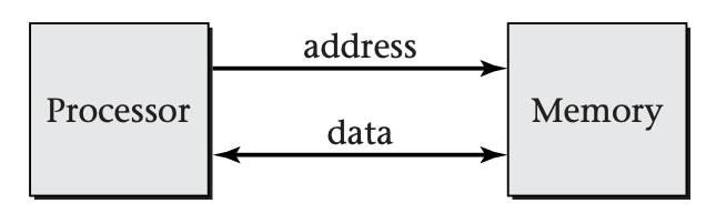
In this system, the processor sends an address to the memory whenever it wants to store a value into memory or load a value from memory. The data being loaded or stored is also transferred in the appropriate direction. Each load operation retrieves the most recent value stored with the specified address. Even though the processor and memory are using a common set of addresses to communicate, the role played by addresses is somewhat different from the perspective of the processor than from the perspective of the memory, as we will now explain.
Addresses from Processor's Perspective
From the perspective of the processor (and the program the processor is executing), addresses are a way of differentiating stored objects from one another. If the processor stores more than one value, and then wishes to retrieve one of those values, it needs to specify which one should be retrieved. Hence, it uses addresses essentially as names. Just as an executive might tell a clerk to "file this under 'widget suppliers' " and then later ask the clerk to "get me that document we filed under 'widget suppliers'," the processor tells the memory to store a value with a particular address and then later loads from that address. Addresses used by executing programs to refer to objects are known as virtual addresses.
Of course, virtual addresses are not arbitrary names; each virtual address is a number. The processor may make use of this to give a group of related objects related names, so that it can easily compute the name of any object in the group. The simplest example of this kind of grouping of related objects is an array. All the array elements are stored at consecutive virtual addresses. That allows the virtual address of any individual element to be computed from the base virtual address of the array and the element's position within the array.
From the memory's perspective, addresses are not identifying names for objects, but rather are spatial locations of storage cells. The memory uses addresses to determine which cells to steer the data into or out of. Addresses used by the memory to specify storage locations are known as physical addresses. The following shows the processor's and memory's views of addresses in a system like that shown above, where the physical addresses come directly from the virtual addresses, and so are numerically equal.
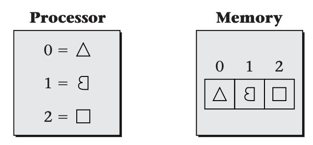
Memory Management Units
The difference between the processor's and memory's perspectives becomes apparent when you consider that the processor may be dividing its time between multiple programs. As we have discussed, the operating system represents running programs as processes. Sometimes the processes will each need a private object, yet the natural name to use will be the same in more than one process. The following figure shows how this necessitates using different addresses in the processor and the memory. That is, virtual addresses can no longer be equal to physical addresses. In this diagram, each process uses the virtual address 0 as a name for its own triangle. This is a simplified model of how more complicated objects are referenced by real processes.
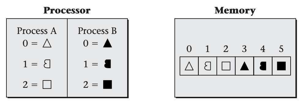
To make this work, general-purpose computers are structured as shown below:
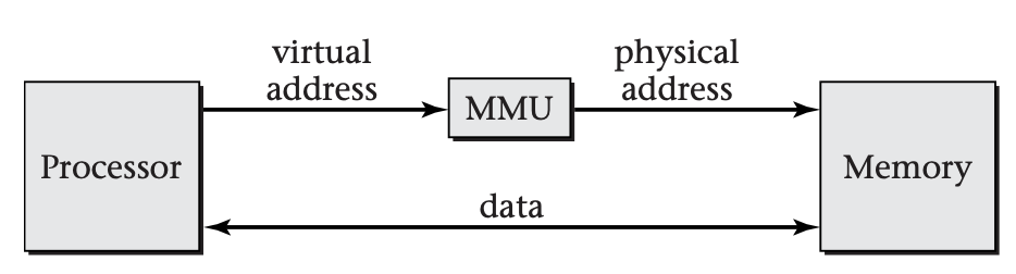
Program execution within the processor works entirely in terms of virtual addresses. However, when a load or store operation is executed, the processor sends the virtual address to an intermediary, the memory management unit (MMU). The MMU translates the virtual address into a corresponding physical address, which it sends to the memory.
Consider next a more realistic example of why each process might use the same virtual addresses for its own objects. Suppose several copies of the same spreadsheet program are running. Each copy will naturally want to refer to "the spreadsheet," but it should be a different spreadsheet object in each process. Even if each process uses a numerical name (that is, a virtual address), it would be natural for all running instances of the spreadsheet program to use the same address; after all, they are running the same code. Yet from the memory's perspective, the different processes' objects need to be stored separately---hence, at different physical addresses.
The same need for private names arises, if not quite so strongly, even if the concurrent processes are running different programs. Although in principle each application program could use different names (that is, virtual addresses) from all other programs, this requires a rather unwieldy amount of coordination.
Even for shared objects, addresses as names behave somewhat differently from addresses as locations. Suppose two processes are communicating via a shared bounded buffer; one is the producer, while the other is the consumer. From the perspective of one process, the buffer is the "output channel," whereas for the other process, it is the "input channel." Each process may have its own name for the object; yet, the memory still needs to store the object in one location. This holds true as well if the names used by the processes are numerical virtual addresses.
Thus, once again, virtual addresses and physical addresses should not be forced to be equal; it should be possible for two processes to use the same virtual address to refer to different physical addresses or to use different virtual addresses to refer to the same physical address.
You have seen that the MMU maps virtual addresses to physical addresses. However, I have not yet discussed the nature of this mapping. So far as anything up to this point goes, the mapping could be as simple as computing each physical address as twice the virtual address. However, that would not yield the very general mechanism known as virtual memory. Instead, virtual memory must have the following additional properties:
-
The function that maps virtual addresses to physical addresses is represented by a table, rather than by a computational rule (such as doubling). That way, the mapping can be much more general and flexible.
-
However, to keep its size manageable, the table does not independently list a physical address for each virtual address. Instead, the virtual addresses are grouped together into blocks known as pages, and the table shows for each page of virtual addresses the corresponding of physical addresses.
-
The contents of the table are controlled by the operating system. This includes both incremental adjustments to the table and wholesale changes of the table when switching between threads. The latter allows each thread to have its own private virtual address space, in which case, the threads belong to different processes.
-
The table need not contain a physical address translation for every page of virtual addresses; in effect, some entries can be left blank. These undefined virtual addresses are illegal for the processor to use. If the processor generates an illegal address, the MMU interrupts the processor, transferring control to the operating system. This interrupt is known as a page fault. This mechanism serves not only to limit the usable addresses but also to allow address translations to be inserted into the table only when needed. By creating address translations in this demand-driven fashion, many applications of virtual memory arrange to move data only when necessary, thereby improving performance.
-
As a refinement of the notion of illegal addresses, some entries in the table may be marked as legal for use, but only in specific ways. Most commonly, it may be legal to read from some particular page of virtual addresses but not to write into that page. The main purpose this serves is to allow trouble-free sharing of memory between processes.
In summary, virtual memory consists of an operating system-defined table of mappings from virtual addresses to physical addresses (at the granularity of pages), with the opportunity for intervention by the operating system on accesses that the table shows to be illegal. You should be able to see that this is a very flexible mechanism. The operating system can switch between multiple views of the physical memory. Parts of physical memory may be completely invisible in some views, because no virtual addresses map to those physical addresses. Other parts may be visible in more than one view, but appearing at different virtual addresses. Moreover, the mappings between virtual and physical addresses need not be established in advance. By marking pages as illegal to access, and then making them available when an interrupt indicates that they are first accessed, the operating system can provide mappings on a demand-driven basis.
Uses for Virtual Memory
This section contains a catalog of uses for virtual memory. The applications of virtual memory enumerated are all in everyday use in most general-purpose operating systems. A comprehensive list would be much longer and would include some applications that have thus far been limited to research systems or other esoteric settings.
Private Storage
The introductory section of this module has already explained that each computation running on a computer may want to have its own private storage, independent of the other computations that happen to be running on the same computer. This goal of private storage can be further elaborated into two subgoals:
-
Each computation should be able to use whatever virtual addresses it finds most convenient for its objects, without needing to avoid using the same address as some other computation.
-
Each computation's objects should be protected from accidental (or malicious) access by other computations.
Both subgoals--independent allocation and protection--can be achieved by giving the computations their own virtual memory mappings. This forms the core of the process concept.
A process is a group of one or more threads with an associated protection context. The phrase "protection context" is intentionally broad, including such protection features as file access permissions. For now, I will focus on one particularly important part of a process's context: the mapping of virtual addresses to physical addresses. In other words, for the purposes of this module, a process is a group of threads that share a virtual address space.
The computer hardware and operating system software collaborate to achieve protection by preventing any software outside the operating system from updating the MMU's address mapping. Thus, each process is restricted to accessing only those physical memory locations that the operating system has allocated as page frames for that process's pages. Assuming that the operating system allocates different processes disjoint portions of physical memory, the processes will have no ability to interfere with one another. The physical memory areas for the processes need only be disjoint at each moment in time; the processes can take turns using the same physical memory.
This protection model, in which processes are given separate virtual address spaces, is the mainstream approach today.
Controlled Sharing
Although the norm is for processes to use disjoint storage, sometimes the operating system will map a limited portion of memory into more than one process's address space. This limited sharing may be a way for the processes to communicate, or it may simply be a way to reduce memory consumption and the time needed to initialize memory. Regardless of the motivation, the shared physical memory can occupy a different range of virtual addresses in each process. (If this flexibility is exercised, the shared memory should not be used to store pointer-based structures, such as linked lists, because pointers are represented as virtual addresses.)
The simplest example of memory-conserving sharing occurs when multiple processes are running the same program. Normally, each process divides its virtual address space into two regions:
-
A read-only region holds the machine language instructions of the program, as well as any read-only data the program contains, such as the character strings printed for error messages. This region is conventionally called the test of the program.
-
A read/write region holds the rest of the process's data. (Many systems actually use two read/write regions, one for the stack and one for other data.)
All processes running the same program can share the same text. The operating system maps the text into each process's virtual memory address space, with the protection bits in the MMU set to enforce read-only access. That way, the shared text does not accidentally become a communication channel.
Interprocess Communication
Modern programs make use of large libraries of supporting code. For example, there is a great deal of code related to graphical user interfaces that can be shared among quite different programs, such as a web browser and a spreadsheet. Therefore, operating systems allow processes to share these libraries with read-only protection, just as for main programs. Microsoft refers to shared libraries as dynamic-link libraries (DLLs).
The below figure illustrates how processes can share in read-only form both program text and the text of DLLs. In this figure, processes A and B are running program 1, which uses DLLs 1 and 2. Processes C and D are running program 2, which uses DLLs 1 and 3. Each process is shown as encompassing the appropriate program text, DLLs, and writable data area. In other words, each process encompasses those areas mapped into its virtual address space.
From the operating system's perspective, the simplest way to support interprocess communication is to map some physical memory into two processes' virtual address spaces with full read/write permissions. Then the processes can communicate freely; each writes into the shared memory and reads what the other one writes. The below figure illustrates this sharing of a writable area of memory for communication.
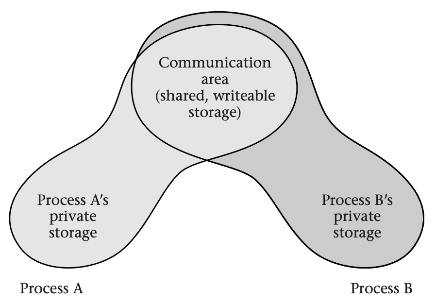
Simple as this may be for the operating system, it is anything but simple for the application programmers. They need to include mutexes, readers-writers locks, or some similar synchronization structure in the shared memory, and they need to take scrupulous care to use those locks. Otherwise, the communicating processes will exhibit races, which are difficult to debug.
Message Passing
Therefore, some operating systems (such as Mac OS X) use virtual memory to support a more structured form of communication, known as message passing, in which one process writes a message into a block of memory and then asks the operating system to send the message to the other process. The receiving process seems to get a copy of the sent message. For small messages, the operating system may literally copy the message from one process's memory to the other's. For efficiency, though, large messages are not actually copied. Instead, the operating system updates the receiver's virtual memory map to point at the same physical memory as the sender's message; thus, sender and receiver both have access to the message, without it being copied. To maintain the ease of debugging that comes from message passing, the operating system marks the page as read-only for both the sender and the receiver. Thus, they cannot engage in any nasty races. Because the sender composes the message before invoking the operating system, the read-only protection is not yet in place during message composition and so does not stand in the way.
As a final refinement to message passing by read-only sharing, systems such as Mac OS X offer copy on write (COW). If either process tries to write into the shared page, the MMU will use an interrupt to transfer control to the operating system. The operating system can then make a copy of the page, so that the sender and receiver now have their own individual copies, which can be writable. The operating system resumes the process that was trying to write, allowing it to now succeed. This provides the complete illusion that the page was copied at the time the message was sent, as shown in this figure:
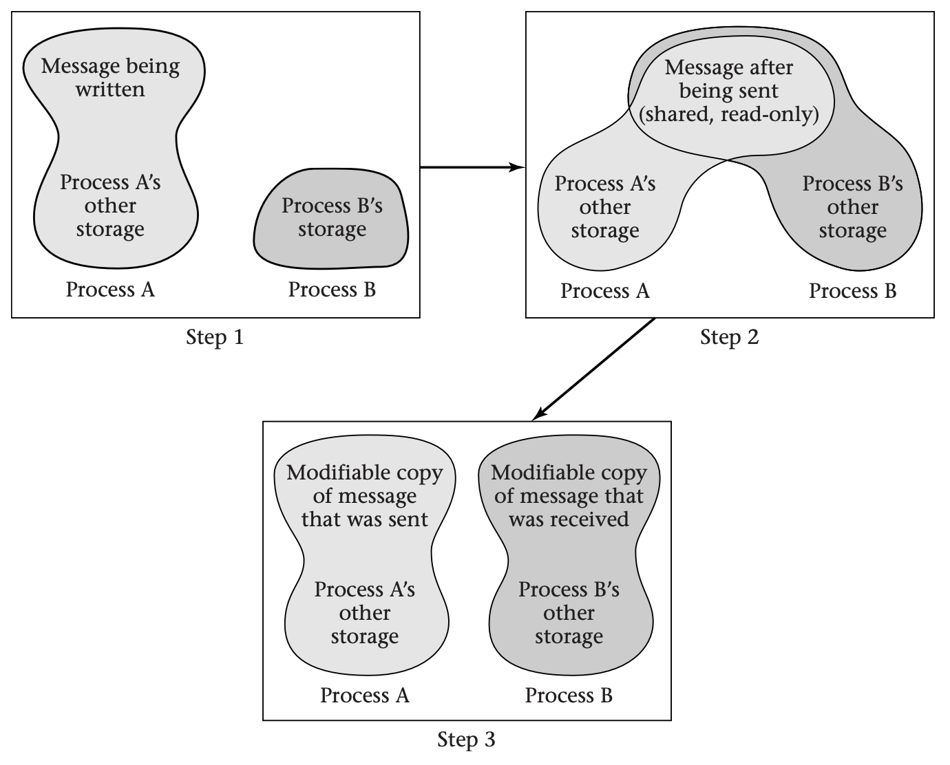
To use copy on write (COW) message passing, process A writes a message into part of its private memory (Step 1) and then asks the operating system to map the memory containing the message into process B’s address space as well (Step 2). Neither process has permission to write into the shared area. If either violates this restriction, the operating system copies the affected page, gives each process write permission for its own copy, and allows the write operation to proceed (Step 3). The net effect is the same as if the message were copied when it was sent, but the copying is avoided if neither process writes into the shared area. The advantage is that if the processes do not write into most message pages, most of the copying is avoided.
Flexible Memory Allocation
The operating system needs to divide the computer's memory among the various processes, as well as retain some for its own use. At first glance, this memory allocation problem doesn't seem too difficult. If one process needs 8 megabytes (MB) and another needs 10, the operating system could allocate the first 8 MB of the memory (with the lowest physical addresses) to the first process and the next 10 MB to the second. However, this kind of contiguous allocation runs into two difficulties.
The first problem with contiguous allocation is that the amount of memory that each process requires may grow and shrink as the program runs. If the first process is immediately followed in memory by the second process, what happens if the first process needs more space?
The second problem with contiguous allocation is that processes exit, and new processes (with different sizes) are started. Suppose you have 512 MB of memory available and three processes running, of sizes 128 MB, 256 MB, and 128 MB. Now suppose the first and third processes terminate, freeing up their 128-MB chunks of memory. Suppose a 256 MB process now starts running. There is enough memory available, but not all in one contiguous chunk, as illustrated below:
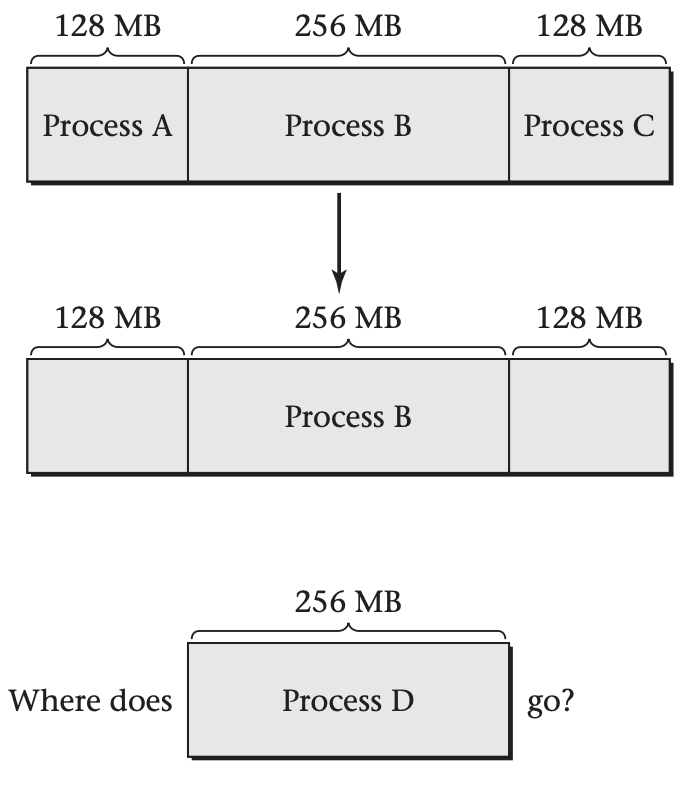
This situation is known as external defragmentation.
Because all modern general-purpose systems have virtual memory, these contiguous allocation difficulties are a non-issue for main memory. The operating system can allocate any available physical page frames to a process, independent of where they are located in memory. For example, the above conundrum of could be solved as shown below:
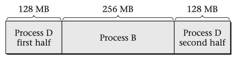
In a more realistic setting, it would be surprising for the pattern of physical memory allocation to display even this degree of contiguity. However, the virtual addresses can be contiguous even if the physical addresses are scattered all over the memory.
Sparse Address Spaces
Just as virtual memory provides the operating system with flexibility in allocating physical memory space, it provides each application program (or process) with flexibility in allocating virtual address space. A process can use whatever addresses make sense for its data structures, even if there are large gaps between them. This provides flexibility for the compiler and runtime environment, which assign addresses to the data structures.
Suppose, for example, that a process has three data structures (S1, S2, and S3) that it needs to store. Each needs to be allocated in a contiguous range of addresses, and each needs to be able to grow at its upper end. The picture might look like this, with addresses in megabytes:
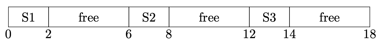
In this example, only one third of the 18-MB address range is actually occupied. If you wanted to allow each structure to grow more, you would have to position them further apart and wind up with an even lower percentage of occupancy. Many real processes span an address range of several gigabytes without using anywhere near that much storage. (Typically, this is done to allow one region to grow up from the bottom of the address space and another to grow down from the top.)
In order to allow processes to use this kind of sparse address space without wastefully occupying a corresponding amount of physical memory, the operating system simply doesn't provide physical address mappings for virtual addresses in the gaps.
Persistence
Any general-purpose operating system must provide some way for users to retain important data even if the system is shut down and restarted. Most commonly, the data is kept in files, although other kinds of persistent objects can be used. The persistent objects are normally stored on disk. For example, as I write this module, I am storing it in files on disk. That way, I don't have to retype the whole module every time the computer is rebooted. So, how does this relate to virtual memory?
When a process needs to access a file (or other persistent object), it can ask the operating system to map the file into its address space. The operating system doesn't actually have to read the whole file into memory. Instead, it can do the reading on a demand-driven basis. Whenever the process accesses a particular page of the file for the first time, the MMU signals a page fault. The operating system can respond by reading that page of the file into memory, updating the mapping information, and resuming the process. (For efficiency reasons, the operating system might choose to fetch additional pages at the same time, on the assumption they are likely to be needed soon.)
If the process writes into any page that is part of a mapped file, the operating system must remember to write the page back to disk, in order to achieve persistence. For efficiency, the operating system should not write back pages that have not been modified since they were last written back or since they were read in. This implies the operating system needs to know which pages have been modified and hence are not up to date on disk. (These are called dirty pages.)
One way to keep track of dirty pages, using only techniques I have already discussed, is by initially marking all pages read-only. That way, the MMU will generate an interrupt on the first attempt to write into a clean page. The operating system can then make the page writable, add it to a list of dirty pages, and allow the operation to continue. When the operating system makes the page clean again, by writing it to disk, it can again mark the page read-only.
Because keeping track of dirty pages is such a common requirement and would be rather inefficient using the approach just described, MMUs generally provide a more direct approach. In this approach, the MMU keeps a dirty bit for each page. Any write into the page causes the hardware to set the dirty bit without needing operating system intervention. The operating system can later read the dirty bits and reset them. (The Intel Itanium architecture contains a compromise: the operating system sets the dirty bits, but with some hardware support. This provides the flexibility of the software approach without incurring so large a performance cost.)
Demand-Driven Program Loading
One particularly important case in which a file gets mapped into memory is running a program. Each executable program is ordinarily stored as a file on disk. Conceptually, running a program consists of reading the program into memory from disk and then jumping to the first instruction.
However, many programs are huge and contain parts that may not always be used. For example, error handling routines will get used only if the corresponding errors occur. In addition, programs often support more features and optional modes than any one user will ever need. Thus, reading in the whole program is quite inefficient.
Even in the rare case that the whole program gets used, an interactive user might prefer several short pauses for disk access to one long one. In particular, reading in the whole program initially means that the program will be slow to start, which is frustrating. By reading in the program incrementally, the operating system can start it quickly at the expense of brief pauses during operation. If each of those pauses is only a few tens of milliseconds in duration and occurs at the time of a user interaction, each will be below the threshold of human perception.
In summary, operating system designers have two reasons to use virtual memory techniques to read in each program on a demand-driven basis: in order to avoid reading unused portions and in order to quickly start the program's execution. As with more general persistent storage, each page fault causes the operating system to read in more of the program.
One result of demand-driven program loading is that application programmers can make their programs start up more quickly by grouping all the necessary code together on a few pages. Of course, laying out the program text is really not a job for the human application programmer, but for the compiler and linker. Nonetheless, the programmer may be able to provide some guidance to these tools.
Efficient Zero Filling
For security reasons, as well as for ease of debugging, the operating system should never let a process read from any memory location that contains a value left behind by some other process that previously used the memory. Thus, any memory not occupied by a persistent object should be cleared out by the operating system before a new process accesses it.
Even this seemingly mundane job--filling a region of memory with zeros--benefits from virtual memory. The operating system can fill an arbitrarily large amount of virtual address space with zeros using only a single zeroed-out page frame of physical memory. All it needs to do is map all the virtual pages to the same physical page frame and mark them as read-only.
In itself, this technique of sharing a page frame of zeros doesn't address the situation where a process writes into one of its zeroed pages. However, that situation can be handled using a variant of the COW technique mentioned previously. When the MMU interrupts the processor due to a write into the read-only page of zeros, the operating system can update the mapping for that one page to refer to a separate read/write page frame of zeros and then resume the process.
If it followed the COW principle literally, the operating system would copy the read-only page frame of zeros to produce the separate, writable page frame of zeros. However, the operating system can run faster by directly writing zeros into the new page frame without needing to copy them out of the read-only page frame. In fact, there is no need to do the zero filling only on demand. Instead, the operating system can keep some spare page frames of zeros around, replenishing the stock during idle time. That way, when a page fault occurs from writing into a read-only page of zeros, the operating system can simply adjust the address map to refer to one of the spare prezeroed page frames and then make it writable.
When the operating system proactively fills spare page frames with zeros during idle time, it should bypass the processor's normal cache memory and write directly into main memory. Otherwise, zero filling can seriously hurt performance by displacing valuable data from the cache.
Substituting Disk Storage for RAM
In explaining the application of virtual memory to persistence, I showed that the operating system can read accessed pages into memory from disk and can write dirty pages back out to disk. The reason for doing so is that disk storage has different properties from main semiconductor memory (RAM). In the case of persistence, the relevant difference is that disk storage is nonvolatile; that is, it retains its contents without power. However, disk differs from RAM in other regards as well. In particular, it is a couple orders of magnitude cheaper per gigabyte. This motivates another use of virtual memory, where the goal is to simulate having lots of RAM using less-expensive disk space. Of course, disk is also five orders of magnitude slower than RAM, so this approach is not without its pitfalls.
Many processes have long periods when they are not actively running. For example, on a desktop system, a user may have several applications in different windows--a word processor, a web browser, a mail reader, a spreadsheet--but focus attention on only one of them for minutes or hours at a time, leaving the others idle. Similarly, within a process, there may be parts that remain inactive. A spreadsheet user might look at the online help once, and then not again during several days of spreadsheet use.
This phenomenon of inactivity provides an opportunity to capitalize on inexpensive disk storage while still retaining most of the performance of fast semiconductor memory. The computer system needs to have enough RAM to hold the working set--the active portions of all active processes. Otherwise, the performance will be intolerably slow, because of disk accesses made on a routine basis. However, the computer need not have enough RAM for the entire storage needs of all the processes: the inactive portions can be shuffled off to disk, to be paged back in when and if they again become active. This will incur some delays for disk access when the mix of activity changes, such as when a user sets the word processor aside and uses a spreadsheet for the first time in days. However, once the new working set of active pages is back in RAM, the computer will again be as responsive as ever.
Much of the history of virtual memory focuses on this one application, dating back to the invention of virtual memory in the early 1960s. (At that time, the two memories were magnetic cores and magnetic drum, rather than semiconductor RAM and magnetic disk.) Even though this kind of paging to disk has become only one of many roles played by virtual memory, I will still pay it considerable attention. In particular, some of the most interesting policy questions arise only for this application of virtual memory. When the operating system needs to free up space in overcrowded RAM, it needs to guess which pages are unlikely to be accessed soon. I will come back to this topic (so-called replacement policies) after first considering other questions of mechanism and policy that apply across the full spectrum of virtual memory applications.
Mechanisms for Virtual Memory
Address mapping needs to be flexible, yet efficient. This means that the mapping function is stored in an explicit table, but at the granularity of pages rather than individual bytes or words. Many systems today use fixed-size pages, perhaps with a few exceptions for the operating system itself or hardware access, though research suggests that more general mixing of page sizes can be beneficial. (Linux has moved in this direction.)
Typical page sizes have grown over the decades; today, the most common is 4 kibibytes (KiB). Each page of virtual memory and each page frame of physical memory is this size, and each starts at an address that is a multiple of the page size. For example, with 4-KiB pages, the first page (or page frame) has address 0, the next has address 4096, then 8192, and so forth.
Each page of virtual memory address space maps to an underlying page frame of physical memory or to none. For example, the following shows one possible mapping, on a system with unrealistically few pages and page frames.
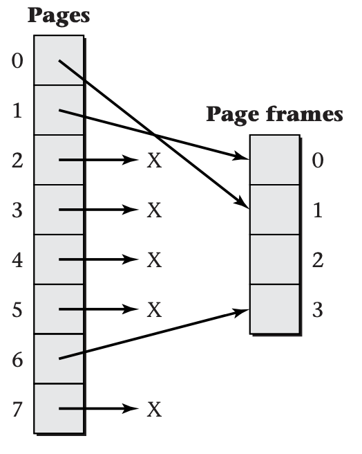
The numbers next to the boxes are page numbers and page frame numbers. The starting addresses are these numbers multiplied by the page size. At the top of this figure, you can see that page 0 is stored in page frame 1. If the page size is 4 KiB, this means that virtual address 0 translates to physical address 4096, virtual address 100 translates to physical address 4196, and so forth. The virtual address of the last 4-byte word in page 0, 4092, translates to the physical address of the last word in page frame 1, 8188. Up until this point, all physical addresses were found by adding 4096 to the virtual address. However, the very next virtual address, 4096, translates to physical address 0, because it starts a new page, which is mapped differently. Note also that page frame 2 is currently not holding any page, and that pages 2--5 and page 7 have no translation available.
Of course, a realistic computer system will have many more page frames of physical memory and pages of virtual address space. Often there are tens or hundreds of thousands of page frames and at least hundreds of thousands of pages. As a result, operating system designers need to think carefully about the data structure used to store the table that maps virtual page numbers to physical page frame numbers. The following will be devoted to presenting three alternative structures that are in current use for page tables: linear, multilevel, and hashed.
Whatever data structure the operating system uses for its page table, it will need to communicate the mapping information to the hardware's MMU, which actually performs the mapping. The nature of this software/hardware interface constrains the page table design and also provides important context for comparing the performance of alternative page table structures.
Software/Hardware Interface
You have seen that the operating system stores some form of page table data structure in memory, showing which physical memory page frame (if any) holds each virtual memory page. Although I will present several possible page table structures shortly, the most important design issue applies equally to all of them: the page table should almost never be used.
Performance considerations explain why such an important data structure should be nearly useless (in the literal sense). Every single memory access performed by the processor generates a virtual address that needs translation to a physical address. Naively, this would mean that every single memory access from the processor requires a lookup operation in the page table. Performing that lookup operation would require at least one more memory access, even if the page table were represented very efficiently. Thus, the number of memory accesses would at least double: for each real access, there would be one page table access. Because memory performance is often the bottleneck in modern computer systems, this means that virtual memory might well make programs run half as fast--unless the page table lookup can be mostly avoided. Luckily, it can.
The virtual addresses accessed by realistic software are not random; instead, they exhibit both temporal locality and spatial locality. That is, addresses that are accessed once are likely to be accessed again before long, and nearby addresses are also likely to be accessed soon. Because a nearby address is likely to be on the same page, both kinds of locality wind up creating temporal locality when considered at the level of whole pages. If a page is accessed, chances are good that the same page will be accessed again soon, whether for the same address or another.
The MMU takes advantage of this locality by keeping a quickly accessible copy of a modest number of recently used virtual-to-physical translations. That is, it stores a limited number of pairs, each with one page number and the corresponding page frame number. This collection of pairs is called the translation lookaside buffer (TLB). Most memory accesses will refer to page numbers present in the TLB, and so the MMU will be able to produce the corresponding page frame number without needing to access the page table. This happy circumstance is known as a TLB hit; the less fortunate case, where the TLB does not contain the needed translation, is a TLB miss.
The TLB is one of the most performance-critical components of a modern microprocessor. In order for the system to have a fast clock cycle time and perform well on small benchmarks, the TLB must be very quickly accessible. In order for the system's performance not to fall off sharply on larger workloads, the TLB must be reasonably large (perhaps hundreds of entries), so that it can still prevent most page table accesses. Unfortunately, these two goals are in conflict with one another: chip designers know how to make lookup tables large or fast, but not both. Coping as well as possible with this dilemma requires cooperation from the designers of hardware, operating system, and application software:
-
The hardware designers ameliorate the problem by including two TLBs, one for instruction fetches and one for data loads and stores. That way, these two categories of memory access don't need to compete for the same TLB.
-
The hardware designers may further ameliorate the problem by including a hierarchy of TLBs, analogous to the cache hierarchy. A small, fast level-one (L1) TLB makes most accesses fast, while a larger, slower level-two (L2) TLB ensures that the page table won't need to be accessed every time the L1 TLB misses. As an example, the AMD Opteron microprocessor contains 40-entry L1 instruction and data TLBs, and it also contains 512-entry L2 instruction and data TLBs.
-
The hardware designers also give the operating system designers some tools for reducing the demand for TLB entries. For example, if different TLB entries can provide mappings for pages of varying sizes, the operating system will be able to map large, contiguously allocated structures with fewer TLB entries, while still retaining flexible allocation for the rest of virtual memory.
-
The operating system designers need to use tools such as variable page size to reduce TLB entry consumption. At a minimum, even if all application processes use small pages (4 KiB), the operating system itself can use larger pages. Similarly, a video frame buffer of many consecutive megabytes needn't be carved up into 4-KiB chunks. As a secondary benefit, using larger pages can reduce the size of page tables. In many cases, smaller page tables are also quicker to access.
-
More fundamentally, all operating system design decisions need to be made with an eye to how they will affect TLB pressure, because this is such a critical performance factor. One obvious example is the normal page size. Another, less obvious, example is the size of the scheduler's time slices: switching processes frequently will increase TLB pressure and thereby hurt performance, even if the TLB doesn't need to be flushed at every process switch. (I will take up that latter issue shortly.)
-
The application programmers also have a role to play. Programs that exhibit strong locality of reference will perform much better, not only because of the cache hierarchy, but also because of the TLB. The performance drop-off when your program exceeds the TLB's capacity is generally quite precipitous. Some data structures are inherently more TLB-friendly than others. For example, a large, sparsely occupied table may perform much worse than a smaller, more densely occupied table. In this regard, theoretical analyses of algorithms may be misleading, if they assume all memory operations take a constant amount of time.
At this point, you have seen that each computer system uses two different representations of virtual memory mappings: a page table and a TLB. The page table is a comprehensive but slow representation, whereas the TLB is a selective but fast representation. You still need to learn how entries from the page table get loaded into the TLB. This leads to the topic of the software/hardware interface.
In general, the MMU loads page table entries into the TLB on a demand-driven basis. That is, when a memory access results in a TLB miss, the MMU loads the relevant translation into the TLB from the page table, so that future accesses to the same page can be TLB hits. The key difference between computer architectures is whether the MMU does this TLB loading autonomously, or whether it does it with lots of help from operating system software running on the processor.
In many architectures, the MMU contains hardware, known as a page table walker, that can do the page table lookup operation without software intervention. In this case, the operating system must maintain the page table in a fixed format that the hardware understands. For example, on an IA-32 processor (such as the Pentium 4), the operating system has no other realistic option than to use a multilevel page table, because the hardware page table walker expects this format. The software/hardware interface consists largely of a single register that contains the starting address of the page table. The operating system just loads this register and lets the hardware deal with loading individual TLB entries. Of course, there are some additional complications. For example, if the operating system stores updated mapping information into the page table, it needs to flush obsolete entries from the TLB.
In other processors, the hardware has no specialized access to the page table. When the TLB misses, the hardware transfers control to the operating system using an interrupt. The operating system software looks up the missing address translation in the page table, loads the translation into the TLB using a special instruction, and resumes normal execution. Because the operating system does the page table lookup, it can use whatever data structure its designer wishes. The lookup operation is done not with a special hardware walker, but with normal instructions to load from memory. Thus, the omission of a page table walker renders the processor more flexible, as well as simpler. However, TLB misses become more expensive, as they entail a context switch to the operating system with attendant loss of cache locality. The MIPS processor, used in the Sony PlayStation 2, is an example of a processor that handles TLB misses in software.
Architectures also differ in how they handle process switches. Recall that each process may have its own private virtual memory address space. When the operating system switches from one process to another, the translation of virtual addresses to physical addresses needs to change as well. In some architectures, this necessitates flushing all entries from the TLB. (There may be an exception for global entries that are not flushed, because they are shared by all processes.) Other architectures tag the TLB entries with a process identifying number, known as an address space identifier (ASID). A special register keeps track of the current process's ASID. For the operating system to switch processes, it simply stores a new ASID into this one register; the TLB need not be flushed. The TLB will hit only if the ASID and page number both match, effectively ignoring entries belonging to other processes.
For those architectures with hardware page table walkers, each process switch may also require changing the register pointing to the page table. Typically, linear page tables and multilevel page tables are per process. If an operating system uses a hashed page table, on the other hand, it may share one table among all processes, using ASID tags just like in the TLB.
Having seen how the MMU holds page translations in its TLB, and how those TLB entries are loaded from a page table either by a hardware walker or operating system software, it is time now to turn to the structure of page tables themselves.
Linear Page Tables
Linear page tables are conceptually the simplest form of page table, though as you will see, they turn out to be not quite so simple in practice as they are in concept. A linear page table is an array with one entry per page in the virtual address space. The first entry in the table describes page 0, the next describes page 1, and so forth. To find the information about page [n], one uses the same approach as for any array access: multiply [n] by the size of a page table entry and add that to the base address of the page table.
Recall that each page either has a corresponding page frame or has none. Therefore, each page table entry contains, at a minimum, a valid bit and a page frame number. If the valid bit is 0, the page has no corresponding frame, and the page frame number is unused. If the valid bit is 1, the page is mapped to the specified page frame. Real page tables often contain other bits indicating permissions (for example, whether writing is allowed), dirtiness, and so forth.
The prior figure showed an example virtual memory configuration in which page 0 was held in page frame 1, page 1 in page frame 0, and page 6 in page frame 3. The figure below shows how this information would be expressed in a linear page table.
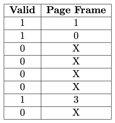
In a linear page table, the information about page [n] is stored at position number [n]>, counting from 0. In this example, the first row, position 0, shows that page 0 is stored in page frame 1. The second-to-last row, position 6, shows that page 6 is stored in page frame 3. The rows with valid bit 0 indicate that no page frame holds the corresponding pages, number 2–5 and 7. In these page table entries, the page frame number is irrelevant and can be any number; an X is shown to indicate this.
Notice that the page numbers are not stored in the linear page table; they are implicit in the position of the entries. The first entry is implicitly for page 0, the next for page 1, and so forth, on down to page 7. If each page table entry is stored in 4 bytes, this tiny page table would occupy 32 consecutive bytes of memory. The information that page 3 has no valid mapping would be found 12 bytes after the base address of the table.
The fundamental problem with linear page tables is that real ones are much larger than this example. For a 32-bit address space with 4-KiB pages, there are [2^{20}] pages, because 12 of the 32 bits are used to specify a location within a page of 4 KiB or [2^{12}] bytes. Thus, if you again assume 4 bytes per page table entry, you now have a 4-MiB page table. Storing one of those per process could use up an undesirably large fraction of a computer's memory. (My computer is currently running 70 processes, for a hypothetical total of 280 MiB of page tables, which would be 36 percent of my total RAM.) Worse yet, modern processors are moving to 64-bit address spaces. Even if you assume larger pages, it is hard to see how a linear page table spanning a 64-bit address space could be stored.
This problem of large page tables is not insurmountable. Linear page tables have been used by 32-bit systems (for example, the VAX architecture, which was once quite commercially important), and even 64-bit linear page tables have been designed--Intel supports them as one option for its current Itanium architecture. Because storing such a huge page table is inconceivable, the secret is to find a way to avoid storing most of the table.
Recall that virtual memory address spaces are generally quite sparse: only a small fraction of the possible page numbers actually have translations to page frames. (This is particularly true on 64-bit systems; the address space is billions of times larger than for 32-bit systems, whereas the number of pages actually used may be quite comparable.) This provides the key to not storing the whole linear page table: you need only store the parts that actually contain valid entries.
On the surface, this suggestion seems to create as big a problem as it solves. Yes, you might now have enough memory to store the valid entries, but how would you ever find the entry for a particular page number? Recall that the whole point of a linear page table is to directly find the entry for page $n$ at the address that is $n$ entries from the beginning of the table. If you leave out the invalid entries, will this work any more? Not if you squish the addresses of the remaining valid entries together. So, you had better not do that.
You need to avoid wasting memory on invalid entries, and yet still be able to use a simple array-indexing address calculation to find the valid entries. In other words, the valid entries need to stay at the same addresses, whether there are invalid entries before them or not. Said a third way, although you want to be thrifty with storage of the page table, you cannot be thrifty with addresses. This combination is just barely possible, because storage and addressing need not be the same.
Divorcing the storage of the page table from the allocation of addresses for its entries requires three insights:
-
The pattern of address space usage, although sparse, is not completely random. Often, software will use quite a few pages in a row, leave a large gap, and then use many more consecutive pages. This clumping of valid and invalid pages means that you can decide which portions of the linear page table are worth storing at a relatively coarse granularity and not at the granularity of individual page table entries. You can store those chunks of the page table that contain any valid entries, even if there are also a few invalid entries mixed in, and not store those chunks that contain entirely invalid entries.
-
In fact, you can choose your chunks of page table to be the same size as the pages themselves. For example, in a system with 4-KiB pages and 4-byte page table entries, each chunk of page table would contain 1024 page table entries. Many of these chunks won't actually need storage, because there are frequently 1024 unused pages in a row. Therefore, you can view the page table as a bunch of consecutive pages, some of which need storing and some of which don't.
-
Now for the trick: use virtual memory to store the page table. That way, you decouple the addresses of page table entries from where they are stored--if anywhere. The virtual addresses of the page table entries will form a nice orderly array, with the entry for page $n$ being $n$ entries from the beginning. The physical addresses are another story. Recall that the page table is divided into page-sized chunks, not all of which you want to store. For those you want to store, you allocate page frames, wherever in memory is convenient. For those you don't want to store, you don't allocate page frames at all.
If this use of virtual memory to store the virtual memory's page table seems dizzying, it should. Suppose you start with a virtual address that has been generated by a running application program. You need to translate it into a physical address. To do so, you want to look up the virtual page number in the page table. You multiply the application-generated virtual page number by the page table entry size, add the base address, and get another virtual address: the virtual address of the page table entry. So, now what? You have to translate the page table entry's virtual address to a physical address. If you were to do this the same way, you would seem to be headed down the path to infinite recursion. Systems that use linear page tables must have a way out of this recursion. Below, the box labeled "?" must not be another copy of the whole diagram. That is where the simple concept becomes a not-so-simple reality.
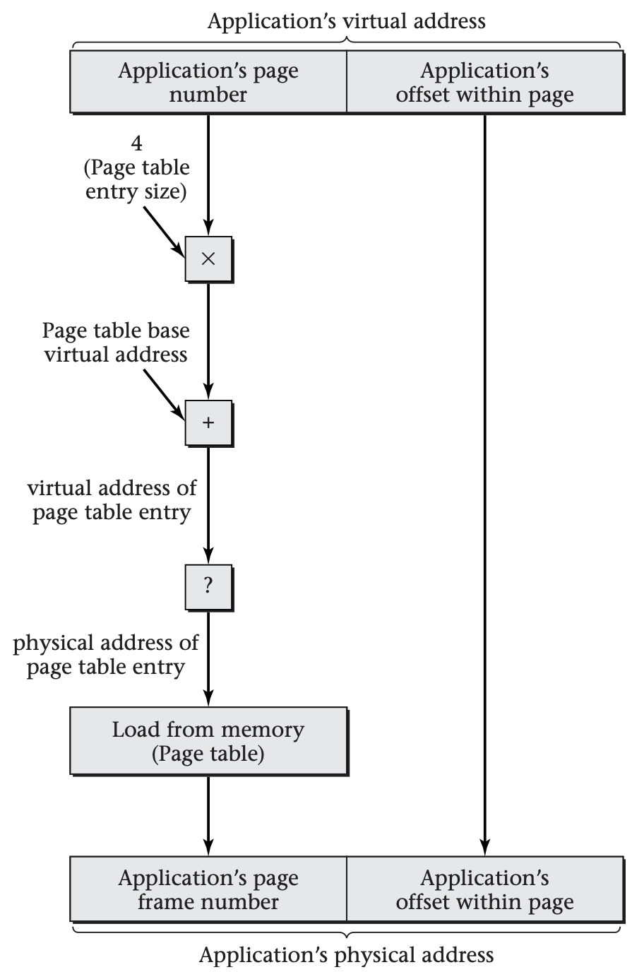
This diagram shows how a virtual address, generated by an application process, is translated into a physical address using a linear page table. At one point in the translation procedure, indicated by a “?” in this diagram, the virtual address of the page table entry needs to be translated into a physical address. This must be done using a method that is different from the one used for the application’s virtual address, in order to avoid an infinite recursion. To see this, imagine inserting another copy of the whole diagram in place of the “?” box. A second “?” would result, which would require further substitution, and so forth to infinity.
Most solutions to the recursion problem take the form of using two different representations to store the virtual-to-physical mapping information. One (the linear page table) is used for application-generated virtual addresses. The other is used for the translation of page table entries' virtual addresses. For example, a multilevel page table accessed using a physical address can be used to provide the mapping information for the pages holding the main linear page table.
This may leave you wondering what the point of the linear page table is. If another representation is going to be needed anyway, why not use it directly as the main page table, for mapping all pages, rather than only indirectly, for mapping the page table's pages? To answer this, you need to recall that the MMU has a TLB in which it keeps track of recently used virtual-to-physical translations; repeated access to the same virtual page number doesn't require access to the page table. Only when a new page number is accessed is the page table (of whatever kind) accessed. This is true not only when translating the application's virtual address, but also when translating the virtual address of a page table entry.
Depending on the virtual address generated by the application software, there are three possibilities:
-
For an address within the same page as another recent access, no page table lookup is needed at all, because the MMU already knows the translation.
-
For an address on a new page, but within the same chunk of pages as some previous access, only a linear page table lookup is needed, because the MMU already knows the translation for the appropriate page of the linear page table.
-
For an address on a new page, far from others that have been accessed, both kinds of page table lookup are needed, because the MMU has no relevant translations cached in its TLB.
Because virtual memory accesses generally exhibit temporal and spatial locality, most accesses fall into the first category. However, for those accesses, the page table organization is irrelevant. Therefore, to compare linear page tables with alternative organizations, you should focus on the remaining accesses. Of those accesses, spatial locality will make most fall into the second category rather than the third. Thus, even if there is a multilevel page table behind the scenes, it will be used only rarely. This is important, because the multilevel page table may be quite a bit slower than the linear one. Using the combination improves performance at the expense of complexity.
Multilevel Page Tables
Recall that the practicality of linear page tables relies on two observations:
-
Because valid page table entries tend to be clustered, if the page table is divided into page-sized chunks, there will be many chunks that don't need storage.
-
The remaining chunks can be located as though they were in one big array by using virtual memory address translation to access the page table itself.
These two observations are quite different from one another. The first is an empirical fact about most present-day software. The second is a design decision. You could accept the first observation while still making a different choice for how the stored chunks are located. This is exactly what happens with multilevel page tables (also known as hierarchical page tables or forward-mapped page tables). They too divide the page table into page-sized chunks, in the hopes that most chunks won't need storage. However, they locate the stored chunks without recursive use of virtual memory by using a tree data structure, rather than a single array.
For simplicity, start by considering the two-level case. This suffices for 32-bit architectures and is actually used in the extremely popular IA-32 architecture, the architecture of Intel's Pentium and AMD's Athlon family microprocessors. The IA-32 architecture uses 4-KiB pages and has page table entries that occupy 4 bytes. Thus, 1024 page-table entries fit within one page-sized chunk of the page table. As such, a single chunk can span 4 MiB of virtual address space. Given that the architecture uses 32-bit virtual addresses, the full virtual address space is 4 gibibytes (GiB) (that is, [2^{32}] bytes); it can be spanned by 1024 chunks of the page table. All you need to do is locate the storage of each of those 1024 chunks or, in some cases, determine that the chunk didn't merit storage. You can do that using a second-level structure, much like each of the chunks of the page table. It, too, is 4 KiB in size and contains 1024 entries, each of which is 4 bytes. However, these entries in the second-level point to the 1024 first-level chunks of the page table, rather than to individual page frames. See below for an illustration of the IA-32 page table's two-level hierarchy, with branching factor 1024 at each level. In this example, page 1 is invalid, as are pages 1024-2047.
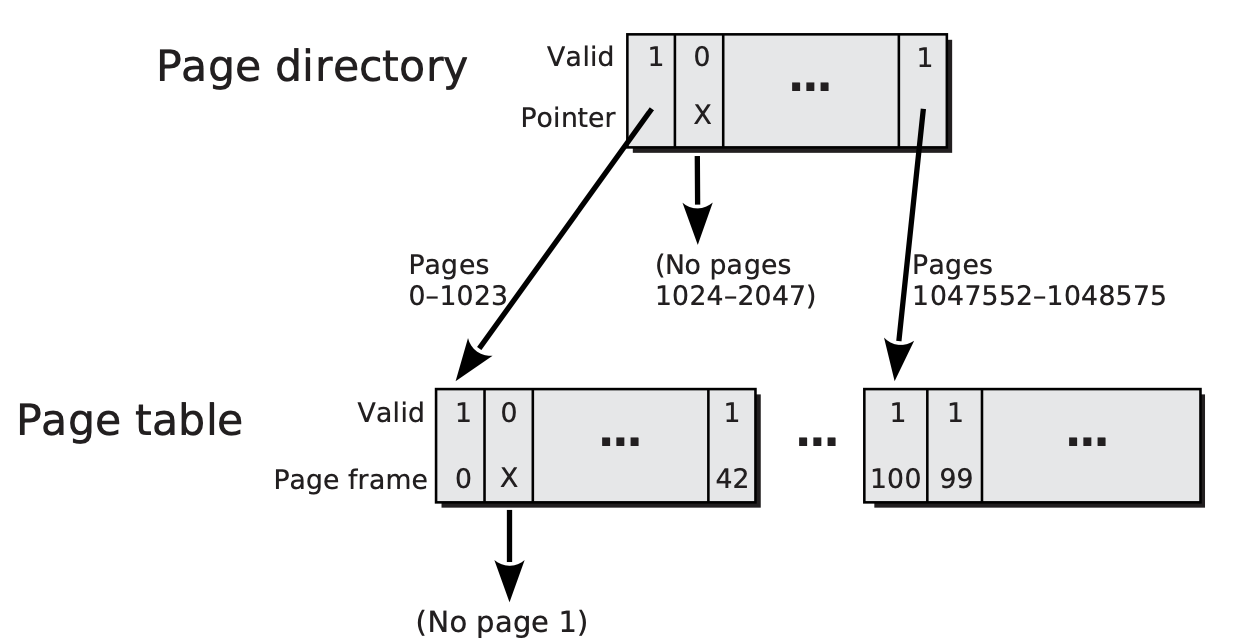
The IA-32 two-level page table has a page directory that can point to 1024 chunks of the page table, each of which can point to 1024 page frames. For example, the leftmost entry of the leftmost chunk of the page table points to the page frame holding page 0, which is page frame 0; besides, page frame 42 holds page 1023, while page frames 100 and 99 hold pages 1047552 and 1047553, respectively. Each entry can also be marked invalid, indicated by a valid bit of 0 and an X in this diagram. For example, the second entry in the first chunk of the page table is invalid, showing that no page frame holds page 1. The same principle applies at the page directory level; in this example, no page frames hold pages 1024–2047, so the second page directory entry is marked invalid.
The operating system on an IA-32 machine stores the physical base address of the page directory in a special register, where the hardware's page table walker can find it. Suppose that at some later point, the processor generates a 32-bit virtual address and presents it to the MMU for translation. The following figure shows the core of the translation process, omitting the TLB and the validity checks.
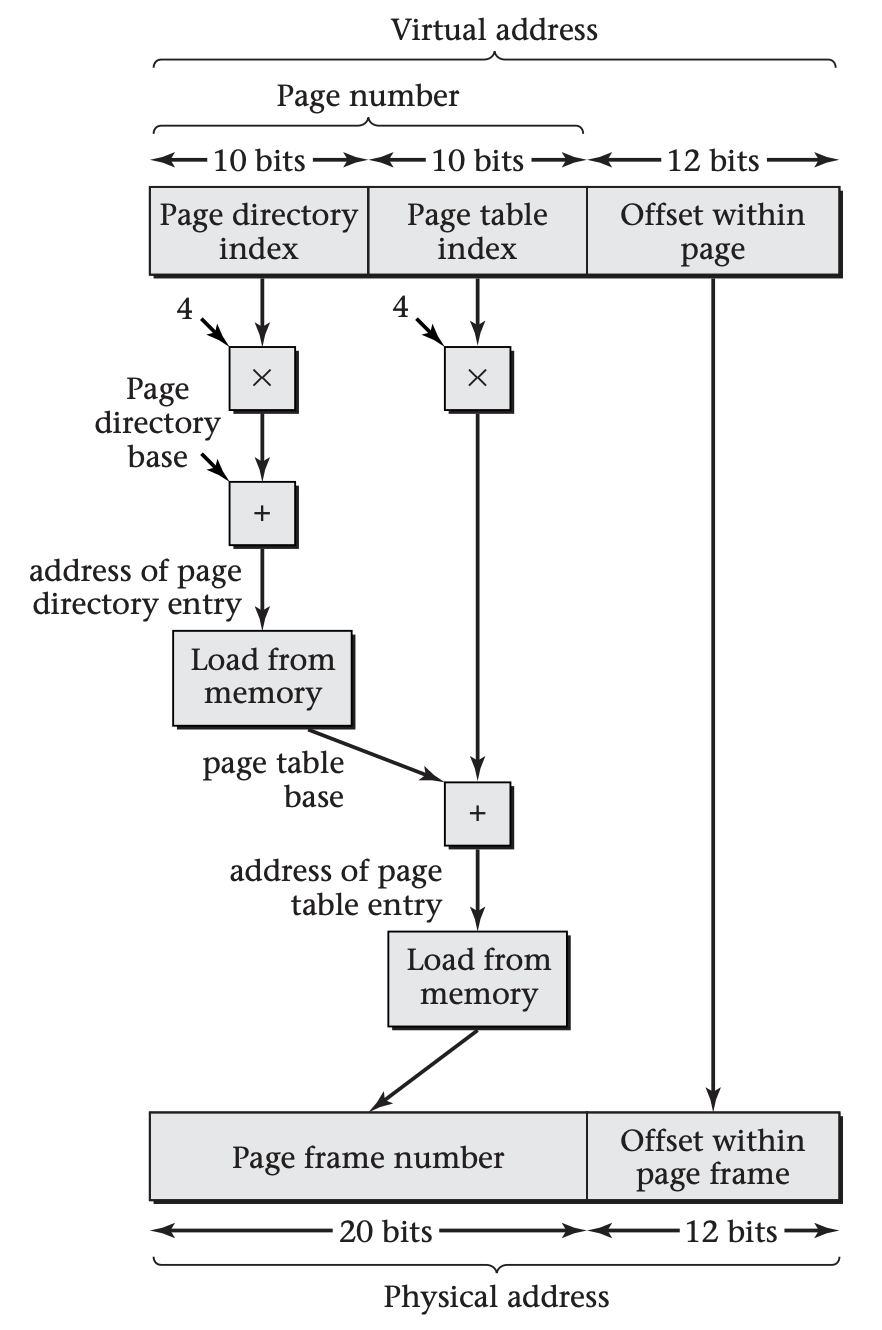
This diagram shows only the core of IA-32 paged address mapping, omitting the TLB and validity checks. The virtual address is divided into a 20-bit page number and 12-bit offset within the page; the latter 12 bits are left unchanged by the translation process. The page number is subdivided into a 10-bit page directory index and a 10-bit page table index. Each index is multiplied by 4, the number of bytes in each entry, and then added to the base physical address of the corresponding data structure, producing a physical memory address from which the entry is loaded. The base address of the page directory comes from a register, whereas the base address of the page table comes from the page directory entry.
In more detail, the MMU follows the following translation process:
-
Initially divide the 32-bit virtual address into its left-hand 20 bits (the page number) and right-hand 12 bits (the offset within the page).
-
Look up the 20-bit page number in the TLB. If a TLB hit occurs, concatenate the resulting page frame number with the 12-bit offset to form the physical address. The process is over.
-
On the other hand, if a TLB miss occurred, subdivide the 20-bit page number into its left-hand 10 bits (the page directory index) and its right-hand 10 bits (the page table index).
-
Load the page directory entry from memory; its address is four times the page directory index plus the page directory base address, which is taken from the special register.
-
Check the page directory entry's valid bit. If it is 0, then there is no page frame holding the page in question--or any of its 1023 neighbors, for that matter. Interrupt the processor with a page fault.
-
Conversely, if the valid bit is 1, the page directory entry also contains a physical base address for a chunk of page table.
-
Load the page table entry from memory; its address is four times the page table index plus the page table base address, which comes from the previous step.
-
Check the page table entry's valid bit. If it is 0, then there is no page frame holding the page in question. Interrupt the processor with a page fault.
-
On the other hand, if the valid bit is 1, the page table entry also contains the physical page frame number. Load the TLB and complete the memory access.
This description, although somewhat simplified, shows the key feature of the IA-32 design: it has a compact page directory, with each entry covering a span of 4 MiB. For the 4-MiB regions that are entirely invalid, nothing further is stored. For the regions containing valid pages, the page directory entry points to another compact structure containing the individual page table entries.
The actual IA-32 design derives some additional advantages from having the page directory entries with their 4-MiB spans:
-
Each page directory entry can optionally point directly to a single large 4-MiB page frame, rather than pointing to a chunk of page table entries leading indirectly to 4-KiB page frames, as I described. This option is controlled by a page-size bit in the page directory entry. By using this feature, the operating system can more efficiently provide the mapping information for large, contiguously allocated structures.
-
Each page directory entry contains permission bits, just like the page table entries do. Using this feature, the operating system can mark an entire 4-MiB region of virtual address space as being read-only more quickly, because it doesn't need to set the read-only bits for each 4-KiB page in the region. The translation process outlined earlier is extended to check the permission bits at each level and signal a page fault interrupt if there is a permission violation at either level.
The same principle used for two-level page tables can be expanded to any greater number of levels. In data structures, you may seethis structure called a trie (or perhaps a radix tree or digital tree). The virtual page number is divided into groups of consecutive bits. Each group of bits forms an index for use at one level of the tree, starting with the leftmost group at the top level. The indexing at each level allows the chunk at the next level down to be located.
For example, the AMD64 architecture (used in the Opteron and Athlon 64 processors and later imitated by Intel under the name IA-32e) employs four-level page tables of this kind. Although the AMD64 is nominally a 64-bit architecture, the virtual addresses are actually limited to only 48 bits in the current version of the architecture. Because the basic page size is still 4 KiB, the rightmost 12 bits are still the offset within a page. Thus, 36 bits remain for the virtual page number. Each page table entry (or similar entry at the higher levels) is increased in size to 8 bytes, because the physical addresses are larger than in IA-32. Thus, a 4-KiB chunk of page table can reference only 512 pages spanning 2 MiB. Similarly, the branching factor at each higher level of the tree is 512. Because 9 bits are needed to select from 512 entries, it follows that the 36-bit virtual page number is divided into four groups of 9 bits each, one for each level of the tree.
Achieving adequate performance with a four-level page table is challenging. The AMD designers will find this challenge intensified if they extend their architecture to full 64-bit virtual addresses, which would require two more levels be added to the page table. Other designers of 64-bit processors have made different choices: Intel's Itanium uses either linear page tables or hashed page tables, and the PowerPC uses hashed page tables.
Hashed Page Tables
You have seen that linear page tables and multilevel page tables have a strong family resemblance. Both designs rely on the assumption that valid and invalid pages occur in large clumps. As a result, each allows you to finesse the dilemma of wanting to store page table entries for successive pages consecutively in memory, yet not wanting to waste storage on invalid entries. You store page table entries consecutively within each chunk of the table and omit storage for entire chunks of the table.
Suppose you take a radical approach and reject the starting assumption. You will still assume that the address space is sparsely occupied; that is, many page table entries are invalid and should not be stored. (After all, no one buys [2^{64}$] scattered randomly throughout the whole address space. This allows greater flexibility for the designers of runtime environments. As a consequence, you will have to store individual valid page table entries, independent of their neighbors.
Storing only individual valid page table entries without storing any of the invalid entries takes away the primary tool used by the previous approaches for locating entries. You can no longer find page $n$'s entry by indexing $n$ elements into an array--not even within each chunk of the address space. Therefore, you need to use an entirely different approach to locating page table entries. You can store them in a hash table, known as a .
A hashed page table is an array of hash buckets, each of which is a fixed-sized structure that can hold some small number of page table entries. (In the Itanium architecture, each bucket holds one entry, whereas in the PowerPC, each bucket holds eight entries.) Unlike the linear page table, this array of buckets does not have a private location for each virtual page number; as such, it can be much smaller, particularly on 64-bit architectures.
Because of this reduced array size, the page number cannot be directly used as an index into the array. Instead, the page number is first fed through a many-to-one function, the hash function. That is, each page gets assigned a specific hash bucket by the hash function, but many different pages get assigned the same bucket. The simplest plausible hash function would be to take the page number modulo the number of buckets in the array. For example, if there are 1000000 hash buckets, then the page table entries for pages 0, 1000000, 2000000, and so forth would all be assigned to bucket 0, while pages 1, 1000001, 2000001, and so forth would all be assigned to bucket 1.
The performance of the table relies on the assumption that only a few of the pages assigned to a bucket will be valid and hence have page table entries stored. That is, the assumption is that only rarely will multiple valid entries be assigned to the same bucket, a situation known as a . To keep collisions rare, the page table size needs to scale with the number of valid page table entries. Luckily, systems with lots of valid page table entries normally have lots of physical memory and therefore have room for a bigger page table.
Even if collisions are rare, there must be some mechanism for handling them. One immediate consequence is that each page table entry will now need to include an indication of which virtual page number it describes. In the linear and multilevel page tables, the page number was implicit in the location of the page table entry. Now, any one of many different page table entries could be assigned to the same location, so each entry needs to include an identifying tag, much like in the TLB.
For an unrealistically small example of using a hashed page table, we can return to the prior example. Suppose you have a hashed page table with four buckets, each capable of holding one entry. Each of the four entries will contain both a virtual page number and a corresponding physical page frame number. If the hash function consists of taking the page number modulo 4, the table would contain approximately the information shown below:
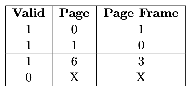
Each entry in a hashed page table is in a location determined by feeding the page number through a hash function. In this example, the hash function consists of taking the page number modulo the number of entries in the table, 4. Consider the entry recording that page 6 is held by page frame 3. This entry is in position 2 within the table (counting from 0) because the remainder when 6 is divided by 4 is 2.
The possibility of collisions has another consequence, beyond necessitating page number tags. Even if collisions occur, each valid page table entry needs to be stored somewhere. Because the colliding entries cannot be stored in the same location, some alternative location needs to be available. One possibility is to have alternative locations within each hash bucket; this is why the PowerPC has room for eight page table entries in each bucket. Provided no collision involves more than this number of entries, they can all be stored in the same bucket. The PowerPC searches all entries in the bucket, looking for one with a matching tag.
If a collision involving more than eight entries occurs on a PowerPC, or any collision at all occurs on an Itanium processor, the collision cannot be resolved within the hash bucket. To handle such collisions, the operating system can allocate some extra memory and chain it onto the bucket in a linked list. This will be an expensive but rare occurrence. As a result, hardware page table walkers do not normally handle this case. If the walker does not find a matching tag within the bucket, it uses an interrupt to transfer control to the operating system, which is in charge of searching through the linked list.
You have now seen two reasons why the page table entries in hashed page tables need to be larger than those in linear or multilevel page tables. The hashed page table entries need to contain virtual page number tags, and each bucket needs a pointer to an overflow chain. As a result of these two factors and the addition of some extra features, the Itanium architecture uses 32-byte entries for hashed page tables versus 8-byte entries for linear page tables.
Incidentally, the fact that the Itanium architecture supports two different page table formats suggests just how hard it is to select one. Research continues into the relative merits of the different formats under varying system workloads. As a result of this research, future systems may use other page table formats beyond those described here, though they are likely to be variants on one of these themes. Architectures such as MIPS that have no hardware page table walker are excellent vehicles for such research, because they allow the operating system to use any page table format whatsoever.
Some operating systems treat a hashed page table as a software TLB, a table similar to the hardware's TLB in that it holds only selected page table entries. In this case, no provision needs to be made for overfull hash buckets; the entries that don't fit can simply be omitted. A slower multilevel page table provides a comprehensive fallback for misses in the software TLB. This alternative is particularly attractive when porting an operating system (such as Linux) that was originally developed on a machine with multilevel page tables.
Policies for Virtual Memory
Thus far, I have defined virtual memory, explained its usefulness, and shown some of the mechanisms typically used to map pages to page frames. Mechanisms alone, however, are not enough. The operating system also needs a set of policies describing how the mechanisms are used. Those policies provide answers for the following questions:
-
At what point is a page assigned a page frame? Not until the page is first accessed, or at some earlier point? This decision is particularly performance critical if the page needs to be fetched from disk at the time it is assigned a page frame. For this reason, the policy that controls the timing of page frame assignment is normally called the fetch policy.
-
Which page frame is assigned to each page? I have said that each page may be assigned any available frame, but some assignments may result in improved performance of the processor's cache memory. The policy that selects a page frame for a page is known as the placement policy.
-
If the operating system needs to move some inactive page to disk in order to free up a page frame, which page does it choose? This is known as the replacement policy, because the page being moved to disk will presumably be replaced by a new page---that being the motivation for freeing a page frame.
All of these policies affect system performance in ways that are quite workload dependent. For example, a replacement policy that performs well for one workload might perform terribly on another; for instance, it might consistently choose to evict a page that is accessed again a moment later. As such, these policies need to be chosen and refined through extensive experimentation with many real workloads. In the following subsections, I will focus on a few sample policies that are reasonably simple and have performed adequately in practice.
Fetch Policy
The operating system has wide latitude regarding when each page is assigned a page frame. At one extreme, as soon as the operating system knows about a page's existence, it could assign a page frame. For example, when a process first starts running, the operating system could immediately assign page frames for all the pages holding the program and its statically allocated data. Similarly, when a process asks the operating system to map a file into the virtual memory address space, the operating system could assign page frames for the entire file. At the other extreme, the operating system could wait for a page fault caused by an access to a page before assigning that page a page frame. In between these extremes lies a range of realistic fetch policies that try to stay just a little ahead of the process's needs.
Creating all page mappings right away would conflict with many of the original goals for virtual memory, such as fast start up of programs that contain large but rarely used portions. Therefore, one extreme policy can be discarded. The other, however, is a reasonable choice under some circumstances. A system is said to use demand paging if it creates the mapping for each page in response to a page fault when accessing that page. Conversely, it uses prepaging if it attempts to anticipate future page use.
Demand paging has the advantage that it will never waste time creating a page mapping that goes unused; it has the disadvantage that it incurs the full cost of a page fault for each page. On balance, demand paging is particularly appropriate under the following circumstances:
-
If the process exhibits limited spatial locality, the operating system is unlikely to be able to predict what pages are going to be used soon. This makes paging in advance of demand less likely to pay off.
-
If the cost of a page fault is particularly low, even moderately accurate predictions of future page uses may not pay off, because so little is gained each time a correct prediction allows a page fault to be avoided.
The Linux operating system uses demand paging in exactly the circumstances suggested by this analysis. The fetch policy makes a distinction between zero-filled pages and those that are read from a file, because the page fault costs are so different. Linux uses demand paging for zero-filled pages because of their comparatively low cost. In contrast, Linux ordinarily uses a variant of prepaging (which I explain in the remainder of this subsection) for files mapped into virtual memory. This makes sense because reading from disk is slow. However, if the application programmer notifies the operating system that a particular memory-mapped file is going to be accessed in a "random" fashion, then Linux uses demand paging for that file's pages. The programmer can provide this information using the madvise procedure.
The most common form of prepaging is clustered paging, in which each page fault causes a cluster of neighboring pages to be fetched, including the one incurring the fault. Clustered paging is also called read round, because pages around the faulting page are read. (By contrast, read ahead reads the faulting page and later pages, but no earlier ones.)
The details of clustered paging vary between operating systems. Linux reads a cluster of sixteen pages aligned to start with a multiple of 16. For example, a page fault on any of the first sixteen pages of a file will cause those sixteen pages to be read. Thus, the extra fifteen pages can be all before the faulting page, all after it, or any mix. Microsoft Windows uses a smaller cluster size, which depends in part on the kind of page incurring the fault: instructions or data. Because instruction accesses generally exhibit more spatial locality than data accesses, Windows uses a larger cluster size for instruction pages than for data pages.
Linux's read around is actually a slight variant on the prepaging theme. When a page fault occurs, the fault handler fetches a whole cluster of pages into RAM but only updates the faulting page table entry. The other pages are in RAM but not mapped into any virtual address space; this status is known as the page cache. Subsequent page faults can quickly find pages in the page cache. Thus, read around doesn't decrease the total number of page faults, but converts many from major page faults (reading disk) to minor page faults (simply updating the page table).
Because reading from disk takes about 10 milliseconds and because reading sixteen pages takes only slightly longer than reading one, the success rate of prepaging doesn't need to be especially high for it to pay off. For example, if the additional time needed to read and otherwise process each prepaged page is half a millisecond, then reading a cluster of sixteen pages, rather than a single page, adds 7.5 milliseconds. This would be more than repaid if even a single one of the fifteen additional pages gets used, because the prepaging would avoid a 10-millisecond disk access time.
Placement Policy
Just as the operating system needs to determine when to make a page resident (on demand or in advance), it needs to decide where the page should reside by selecting one of the unused page frames. This choice influences the physical memory addresses that will be referenced and can thereby influence the miss rate of the cache memory hardware.
Although cache performance is the main issue in desktop systems, there are at least two other reasons why the placement policy may matter. In large-scale multiprocessor systems, main memory is distributed among the processing nodes. As such, any given processor will have some page frames it can more rapidly access. Microsoft's Windows Server 2003 takes this effect into account when allocating page frames. Another issue, likely to become more important in the future, is the potential for energy savings if all accesses can be confined to only a portion of memory, allowing the rest to be put into standby mode.
To explain why the placement policy influences cache miss rate, I need to review cache memory organization. An idealized cache would hold the [n] most recently accessed blocks of memory, where [n] is the cache's size. However, this would require each cache access to examine all [n] blocks, looking to see if any of them contains the location being accessed. This approach, known as full associativity, is not feasible for realistically large caches. Therefore, real caches restrict any given memory location to only a small set of positions within the cache; that way, only those positions need to be searched. This sort of cache is known as set-associative. For example, a two-way set-associative cache has two alternative locations where any given memory block can be stored. Many caches, particularly those beyond the first level (L1), use the physical address rather than the virtual address to select a set.
Consider what would happen if a process repeatedly accesses three blocks of memory that have the misfortune of all competing for the same set of a two-way set-associative cache. Even though the cache may be large--capable of holding far more than the three blocks that are in active use--the miss rate will be very high. The standard description for this situation is to say the cache is suffering from conflict misses rather than capacity misses. Because each miss necessitates an access to the slower main memory, the high rate of conflict misses will significantly reduce performance.
The lower the cache's associativity, the more likely conflict misses are to be a problem. Thus, careful page placement was more important in the days when caches were external to the main microprocessor chips, as external caches are often of low associativity. Improved semiconductor technology has now allowed large caches to be integrated into microprocessors, making higher associativity economical and rendering placement policy less important.
Suppose, though, that an operating system does wish to allocate page frames to reduce cache conflicts. How should it know which pages are important to keep from conflicting? One common approach is to assume that pages that would not conflict without virtual memory address translation should not conflict even with address translation; this is known as . Another common approach is to assume that pages that are mapped into page frames soon after one another are likely to also be accessed in temporal proximity; therefore, they should be given nonconflicting frames. This is known as bin hopping.
The main argument in favor of page coloring is that it leaves intact any careful allocation done at the level of virtual addresses. Some compiler authors and application programmers are aware of the importance of avoiding cache conflicts, particularly in high-performance scientific applications, such as weather forecasting. For example, the compiler or programmer may pad each row of an array with a little wasted space so that iterating down a column of the array won't repeatedly access the same set of the cache. This kind of cache-conscious data allocation will be preserved by page coloring.
The main argument in favor of bin hopping is that experimental evidence suggests it performs better than page coloring does, absent cache-conscious data allocation. This may be because page coloring is less flexible than bin hopping, providing only a way of deciding on the most preferred locations in the cache for any given page, as opposed to ranking all possible locations from most preferred to least.
Replacement Policy
Conceptually, a replacement policy chooses a page to evict every time a page is fetched with all page frames in use. However, operating systems typically try do some eviction in advance of actual demand, keeping an inventory of free page frames. When the inventory drops below a low-water mark, the replacement policy starts freeing up page frames, continuing until the inventory surpasses a high-water mark. Freeing page frames in advance of demand has three advantages:
-
Last-minute freeing in response to a page fault will further delay the process that incurred the page fault. In contrast, the operating system may schedule proactive work to maintain an inventory of free pages when the hardware is otherwise idle, improving response time and throughput.
-
Evicting dirty pages requires writing them out to disk first. If the operating system does this proactively, it may be able to write back several pages in a single disk operation, making more efficient use of the disk hardware.
-
In the time between being freed and being reused, a page frame can retain a copy of the page it most recently held. This allows the operating system to inexpensively recover from poor replacement decisions by retrieving the page with only a minor page fault instead of a major one. That is, the page can be retrieved by mapping it back in without reading it from disk. You will see that this is particularly important if the MMU does not inform the replacement policy which pages have been recently referenced.
In a real operating system, a page frame may go through several temporary states between when it is chosen for replacement and when it is reused. For example, Microsoft Windows may move a replaced page frame through the following four inventories of page frames, as illustrated below:
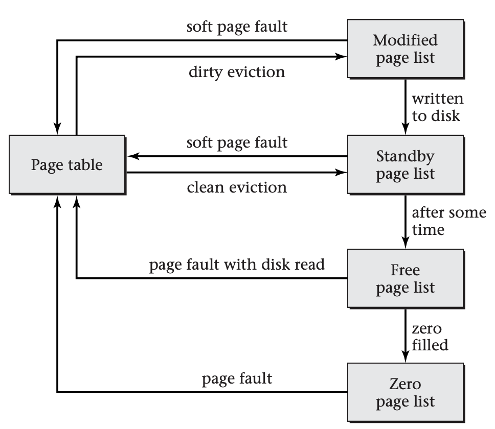
Each page frame in Microsoft Windows that is not referenced from a page table is included in one of the four page lists. Page frames circulate as shown here. For example, the system can use a soft page fault to recover a page frame from the modified or standby page list, if the page contained in that page frame proves to still be needed after having been evicted by the replacement policy.
-
When the replacement policy first chooses a dirty page frame, the operating system moves the frame from a process's page table to the modified page list. The modified page list retains information on the previous page mapping so that a minor page fault can retrieve the page. (Microsoft calls this a soft page fault.)
-
If a page frame remains in the modified page list long enough, a system thread known as the modified page writer will write the contents out to disk and move the frame to the standby page list. A page frame can also move directly from a process's page table to the standby page list if the replacement policy chooses to evict a clean page. The standby page list again retains the previous mapping information so that a soft page fault can inexpensively recover a prematurely evicted page.
-
If a page frame remains on standby for long enough without being faulted back into use, the operating system moves it to the free page list. This list provides page frames for the system's zero page thread to proactively fill with zeros, so that zero-filled pages will be available to quickly respond to page faults, as discussed earlier. The operating system also prefers to use a page frame from the free list when reading a page in from disk.
-
Once the zero page thread has filled a free page frame with zeros, it moves the page frame to the zero page list, where it will remain until mapped back into a process's page table in response to a page fault.
Using a mechanism such as this example from Windows, an operating system keeps an inventory of page frames and thus need not evict a page every time it fetches a page. In order to keep the size of this inventory relatively stable over the long term, the operating system balances the rate of page replacements with the rate of page fetches. It can do this in either of two different ways, which lead to the two major categories of replacement policies, local replacement and global replacement.
Local replacement keeps the rate of page evictions and page fetches balanced individually for each process. If a process incurs many page faults, it will have to relinquish many of its own page frames, rather than pushing other processes' pages out of their frames. The replacement policy chooses which page frames to free only from those held by a particular process. A separate allocation policy decides how many page frames each process is allowed.
Global replacement keeps the rate of page evictions and page fetches balanced only on a system-wide basis. If a process incurs many page faults, other process's pages may be evicted from their frames. The replacement policy chooses which page frames to free from all the page frames, regardless which processes they are used by. No separate page frame allocation policy is needed, because the replacement policy and fetch policy will naturally wind up reallocating page frames between processes.
Of the operating systems popular today, Microsoft Windows uses local replacement, whereas all the members of the UNIX family, including Linux and Mac OS X, use global replacement. Microsoft's choice of a local replacement policy for Windows was part of a broader pattern of following the lead of Digital Equipment Corporation's VMS operating system, which has since become HP's OpenVMS. The key reason why VMS's designers chose local replacement was to prevent poor locality of reference in one process from greatly hurting the performance of other processes. Arguably, this performance isolation is less relevant for a typical Windows desktop or server workload than for VMS's multi-user real-time and timesharing workloads. Global replacement is simpler, and it more flexibly adapts to processes whose memory needs are not known in advance. For these reasons, it tends to be more efficient.
Both local and global replacement policies may be confronted with a situation where the total size of the processes' working sets exceeds the number of page frames available. In the case of local replacement, this manifests itself when the allocation policy cannot allocate a reasonable number of page frames to each process. In the case of global replacement, an excessive demand for memory is manifested as thrashing, that is, by the system spending essentially all its time in paging and process switching, producing extremely low throughput.
The traditional solution to excess memory demand is swapping. The operating system picks some processes to evict entirely from memory, writing all their data to disk. Moreover, it removes those processes' threads from the scheduler's set of runnable threads, so that they will not compete for memory space. After running the remaining processes for a while, the operating system swaps some of them out and some of the earlier victims back in. Swapping adds to system complexity and makes scheduling much choppier; therefore, some global replacement systems such as Linux omit it and rely on users to steer clear of thrashing. Local replacement systems such as Microsoft Windows, on the other hand, have little choice but to include swapping. For simplicity, I will not discuss swapping further in this text. You should know what it is, however, and should also understand that some people incorrectly call paging swapping; for example, you may hear of Linux swapping, when it really is paging. That is, Linux is moving individual pages of a process's address space to disk and back, rather than moving the entire address space.
Having seen some of the broader context into which replacement policies fit, it is time to consider some specific policies. I will start with one that is unrealistic but which provides a standard against which other, more realistic policies can be measured. If the operating system knew in advance the full sequence of virtual memory accesses, it could select for replacement the page that has its next use furthest in the future. This turns out to be more than just intuitively appealing: one can mathematically prove that it optimizes the number of demand fetches. Therefore, this replacement policy is known as optimal replacement (OPT).
Real operating systems don't know future page accesses in advance. However, they may have some data that allows the probability of different page accesses to be estimated. Thus, a replacement policy could choose to evict the page estimated to have the longest time until it is next used. As one special case of this, consider a program that distributes its memory accesses across the pages randomly but with unequal probabilities, so that some pages are more frequently accessed than others. Suppose that these probabilities shift only slowly. In that case, pages which have been accessed frequently in the recent past are likely to be accessed again soon, and conversely, those that have not been accessed in a long while are unlikely to be accessed soon. As such, it makes sense to replace the page that has gone the longest without being accessed. This replacement policy is known as Least Recently Used (LRU).
LRU replacement is more realistic than OPT, because it uses only information about the past, rather than about the future. However, even LRU is not entirely realistic, because it requires keeping a list of page frames in order by most recent access time and updating that list on every memory access. Therefore, LRU is used much as OPT is, as a standard against which to compare other policies. However, LRU is not a gold standard in the same way that OPT is; while OPT is optimal among all policies, LRU may not even be optimal among policies relying only on past activity. Real processes do not access pages randomly with slowly shifting probability distributions. For example, a process might repeatedly loop through a set of pages, in which case LRU will perform terribly, replacing the page that will be reused soonest. Nonetheless, LRU tends to perform reasonably well in many realistic settings; therefore, many other replacement policies try to approximate it. While they may not replace the least recently used page, they will at least replace a page that hasn't been used very recently.
Before considering realistic policies that approximate LRU, I should introduce one other extremely simple policy, which can serve as a foundation for an LRU-approximating policy, though it isn't one itself. The simple policy is known as first in, first out (*FIFO). The name tells the whole story: the operating system chooses for replacement whichever page frame has been holding its current page the longest. Note the difference between FIFO and LRU; FIFO chooses the page that was fetched the longest ago, even if it continues to be in frequent use, whereas LRU chooses the page that has gone the longest without access. The figure below shows an example where LRU outperforms FIFO and is itself outperformed by OPT.
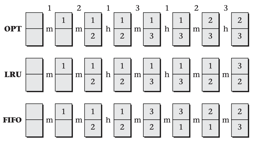
In this comparison of the OPT, LRU, and FIFO replacement policies, each pair of boxes represents the two page frames available on an unrealistically small system. The numbers within the boxes indicate which page is stored in each page frame. The numbers across the top are the reference sequence, and the letters h and m indicate hits and misses. In this example, LRU performs better than FIFO, in that it has one more hit. OPT performs even better, with three hits.
FIFO is not a very smart policy; in fact, early simulations showed that it performs comparably to random replacement. Beyond this mediocre performance, one sign that FIFO isn't very smart is that it suffers from Belady's anomaly: increasing the number of page frames available may increase the number of page faults, rather than decreasing it as one would expect.
Both OPT and LRU are immune from Belady's anomaly, as are all other members of the class of stack algorithms. A stack algorithm is a replacement policy with the property that if you run the same sequence of page references on two systems using that replacement policy, one with [n] page frames and the other with [n+1], then at each point in the reference sequence the [n] pages that occupy page frames on the first system will also be resident in page frames on the second system. For example, with the LRU policy, the [n] most recently accessed pages will be resident in one system, and the [n+1] most recently accessed pages will be resident in the other. Clearly the [n+1] most recently accessed pages include the [n] most recently accessed pages.
Recall that at the beginning of this subsection, I indicated that page frames chosen for replacement are not immediately reused, but rather enter an inventory of free page frames. The operating system can recover a page from this inventory without reading from disk, if the page is accessed again before the containing page frame is reused. This refinement turns out to dramatically improve the performance of FIFO. If FIFO evicts a page that is frequently used, chances are good that it will be faulted back in before the page frame is reused. At that point, the operating system will put it at the end of the FIFO list, so it will not be replaced again for a while. Essentially, the FIFO policy places pages on probation, but those that are accessed while on probation aren't actually replaced. Thus, the pages that wind up actually replaced are those that were not accessed recently, approximating LRU. This approximation to LRU, based on FIFO, is known as Segmented FIFO (SFIFO).
To enable smarter replacement policies, some MMUs provide a in each page table entry. Every time the MMU translates an address, it sets the corresponding page's reference bit to 1. (If the address translation is for a write to memory, the MMU also sets the dirty bit that I mentioned earlier.) The replacement policy can inspect the reference bits and set them back to 0. In this way, the replacement policy obtains information on which pages were recently used. Reference bits are not easy to implement efficiently, especially in multiprocessor systems; thus, some systems omit them. However, when they exist, they allow the operating system to find whether a page is in use more cheaply than by putting it on probation and seeing whether it gets faulted back in.
One replacement policy that uses reference bits to approximate LRU is clock replacement. In clock replacement, the operating system considers the page frames cyclically, like the hand of a clock cycling among the numbered positions. When the replacement policy's clock hand is pointing at a particular page, the operating system inspects that page's reference bit. If the bit is 0, the page has not been referenced recently and so is chosen for replacement. If the bit is 1, the operating system resets it to 0 and moves the pointer on to the next candidate. That way, the page has a chance to prove its utility, by having its reference bit set back to 1 before the pointer comes back around. As a refinement, the operating system can also take the dirty bit into account, as follows:
-
reference = 1: set reference to 0 and move on to the next candidate
-
reference = 0 and dirty = 0: choose this page for replacement
-
reference = 0 and dirty = 1: start writing the page out to disk and move on to the next candidate; when the writing is complete, set dirty to 0
Replacement policies such as FIFO and clock replacement can be used locally to select replacement candidates from within a process, as well as globally. For example, some versions of Microsoft Windows use clock replacement as the local replacement policy on systems where reference bits are available, and FIFO otherwise.
Assignment 7: Virtual Memory
In this activity, you may work in pairs or individually. You may not use ChatGPT or similar tools in any way, shape, or form on this activity. If there is any indication that one of those tools was used, you will received an automatic zero. Instead, working with your peer to do your best answering the questions throughout. Many of the questions are are open-ended, and thus have many possible answers, so I would expect them to vary widely between submissions.
Learning Objectives
Students will be able to…
- Demonstrate an understanding of the process of handling a page fault.
- Articulate the need for a page replacement algorithm in an operating system.
- Compute how many page faults occur for FIFO, OPT, LRU, and Working Set algorithms, for various inputs.
- Articulate the meaning of Belady’s Anomaly.
Instructions
For this assignment, you will complete the worksheet linked below covering topics on System Calls and Processes. You will make a copy of the worksheet and complete your work within your worksheet copy. Note that if you are working with a partner, you will only submit one copy of the worksheet between the two of you.
As with the previous assignment, I encourage you to spend some time thinking through these questions, working them out of paper (making notes and drawing pictures, where necessary). Though there are a lot of questions, no single question should take that much time. If you have done your reading, and think through the models that are provided, you should be able to answer them relatively quickly.
📄 Link to the Worksheet in Google Docs: Google Docs Link
Submitting Your Work
Your work must be submitted to Anchor for degree credit and to Gradescope for grading.
- Complete the work in your copy of the Google Doc.
- After you have completed your answers, export it as a pdf document.
- Submit your pdf document to Gradescope using the appropriate link (one one person per pair needs to upload).
- Upload the pdf document to Anchor using the form below (both individuals must upload their own copy to Anchor).
This assignments is used with permission: © Victor Norman at Calvin University, 2023 vtn2@calvin.edu Version 2.1.1 This work is licensed under the Creative Commons Attribution 4.0 International License. To view a copy of this license, visit http://creativecommons.org/licenses/by/4.0/ or send a letter to Creative Commons, PO Box 1866, Mountain View, CA 94042, USA.
Week 10 Participation
During the live class session this week, you will be asked to complete some of the problems that we went through in this material.
Your completion of these questions and answers, and your engagement during the live class will make up your Weekly Participation Score.