Markov Decision Processes
Now that we have learned about the Reinforcement Learning (RL) framework, let's discuss how we can formulate a problem as an RL problem using the Markov Decision Process (MDP) formalism.
Markov Decision Processes (MDPs) provide a mathematical framework for modeling decision making in situations where outcomes are partly random and partly under the control of a decision maker.
The word "Markov" in MDP refers to the fact that the future can be determined only from the present state (i.e., the future is independent of the past).
A Markov decision process formalism consists of the following elements:
-
A set of states s ∈ S: The different states the agent/world can be in. For example, in autonomous helicopter flight, the states might be the set of all possible positions and orientations of the helicopter. In a simple grid world, the states might be the set of all possible positions (cells) of the robot.
-
A set of actions (A): The set of actions the agent can take. For example, the set of all possible directions in which you can push the helicopter’s control sticks or move the robot in the grid world (
up,down,left,right). -
A reward function R: The reward function is a function of the state. It returns the reward value of being in a state
s. The notation for the reward function isR(s),R(s,a), or R(s,a,s').s'is the state you reach after taking an action a while being in a states. -
A transition probability model Pa(s,s'): is the probability of reaching the next state
s'(pronounced s-prime) if we take actionawhile being in states. Sometimes, the transition probability model is notated asP(s'|s,a)orT(s,a, s'). You can think of it as the model of the world.In the helicopter flight example, if the helicopter is in state
sand we push the control sticks in a certain direction, the helicopter will move in that direction with some probability as the helicopter might be affected by the wind.If a robot is moving in a simple grid world, being in a certain position/cell let's say cell
1,2and you want to move it to position2,2. The world grid model might tell us that each action you take has an0.8probability of being executed successfully. So, when we direct the robot to move up, the robot might move up with a probability of0.8, move right with a probability of0.1, or move left with a probability of0.1.
Simple Grid World Example
To explain the MDP formalism, let's consider a simple MDP. The agent is in a grid world and can move up, down, left, or right. The agent receives a reward of -0.2 for each step and a reward of 10 for reaching the goal. The agent receives a reward of -5 for reaching the cliff. The agent can't move outside the grid world and can't move into the wall.
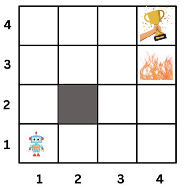
What are the elements of the MDP for this grid world?
-
States are the 15 cells in the grid world. State (2,2) is blocked.
-
Actions are the four directions the agent can move (up, down, left, right).
-
Transition Probability: In this example, we will model our world such that the agent will move in the direction it chooses with probability
0.8. The agent will move in a random direction with probability0.2. For example, if the agent chooses to move up, it will move up with probability0.8and move left or right with probability0.1each. So, the transition probability model is as follows:P(s' = (1, 2) | s = (1, 1), a = up) = 0.8: Being at state (1, 1) and taking action up, the probability of ending up at state (1, 2) is 0.8.P(s' = (1, 1) | s = (1, 1), a = up) = 0.1: Being at state (1, 1) and taking action up, the probability of ending up at state (1, 1) is 0.1.P(s' = (0, 1) | s = (1, 1), a = up) = 0.1: Being at state (1, 1) and taking action up, the probability of ending up at state (0, 1) is 0.1.
-
Reward Function: To incentivize the robot to reach the goal cell, we will put a
+10reward there. Also, to discourage the robot from falling off the cliff, we will put a-5reward there. The robot will receive a-0.2reward for each step.R(s) =-0.2for all states except the goal and the cliff.
The -0.2
is like charging the robot for each step it takes.
The robot should try to minimize the number of steps
it takes to reach the goal.
Policy
The goal of the Markov Decision Process is to find a good policy π for the decision maker. A policy is a function that maps states to actions (π: S → A). The policy tells the agent what action to take in each state. The goal is to find the policy that maximizes the expected total reward.
Optimal Policy: The optimal policy is the policy that maximizes the expected total reward. The optimal policy is denoted by π*. Below is an example of an optimal policy.
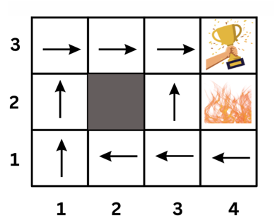
What this policy says is, for example, if the agent is at state (2,1), it should go left. That is π(2,1) = left
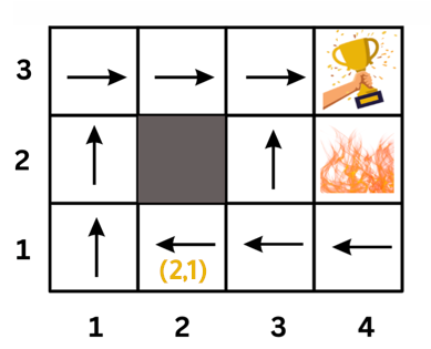
An interesting position to examine in the previous policy is position (3,1). You might think that the optimal policy is to go up because that path is shorter. However, if the agent goes up, there is a 0.1 probability that it will end up at the cliff (moving right after moving up). So the safer path is to go left and then up.
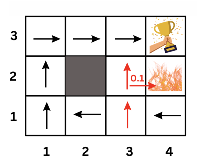
Note that this policy is heavily dependant on the transition probabilities we assumed for our world. If the transition probabilities change, the optimal policy could change too.
Solving the MDP problem is finding the optimal policy.
Markov Decision Process (MDP) Videos:
Here are some (optional) videos that explain the same concepts above. If you feel you need more explanation, you can watch them.
Discount Factor (γ)
Another important concept in MDPs is discounting. It addresses the fact that future rewards are worth less than immediate rewards. It is reasonable for agents to prefer immediate rewards over future rewards and to look forward to maximizing their total reward.
In MDPs, we use a discount factor γ (gamma) to discount future rewards. It is a value between 0 and 1 and it decays after each step.
Here is a formula that shows how the discount factor is used to calculate the expected total reward:
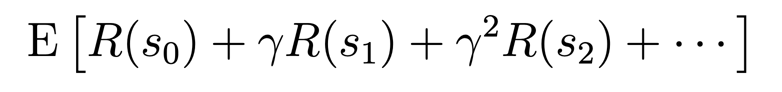
E is the expected total reward the agent will receive if it starts at state s0.
Note that we don't discount the immediate reward R(s0). We discount the future rewards by multiplying them by multiples of γ. the discount factor value decays after each step by multiplying the future rewards by multiples of γ: γ, γ^2, γ^3, γ^4, and so on.
Example:
- If we have a sequence of rewards:
r0 = 1,r1 = 2, andr2 = 3, what is the expected total utility of this sequence of rewards if:- No discounting is used?
- If
γ = 0.5?
Click here to see the answer
-
If no discounting is used, the expected total utility is
1 + 2 + 3 = 6. -
If
γ = 0.5, the expected total utility is1 + 2*0.5 + 3*0.5^2 = 2.75.
Discounting Quiz:
In the image below, we have 5 states: a, b, c, d, and e. The reward function is R(s) = 0 for all states except a and e. R(a) = 10 and R(e) = 1. You can move right or left.
You can also exit from state a or e. The environment is deterministic (transition probability is 1). Answer the questions below.
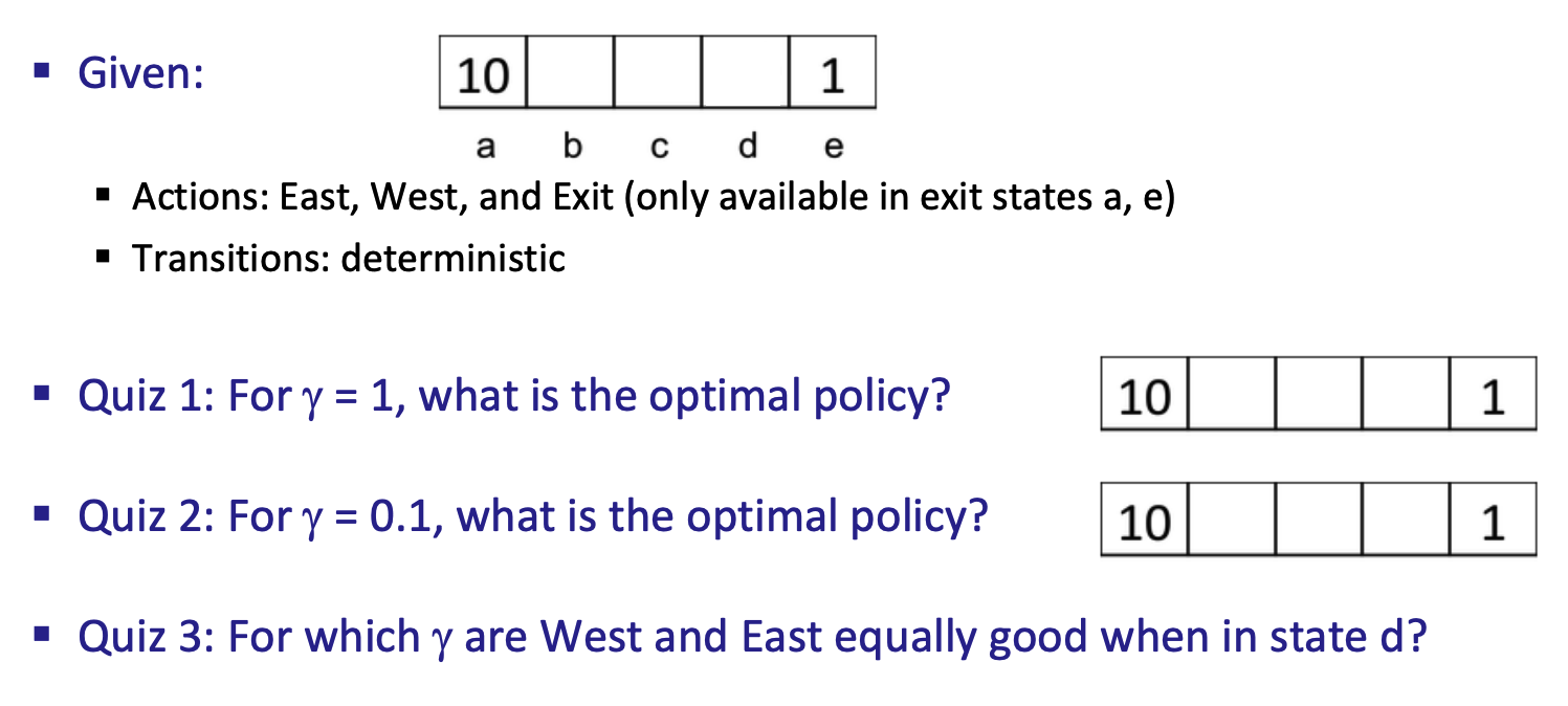
Reference: Berkeley CS188 Intro to AI
- Your answer should be in the form of a policy. For example, if you are at state
b, you should moveleft. If you are at statec, you should moverightetc. Think about the total reward you will get at each state taking into account the discount factorY.
Click here to see the answers
Q1: For Y = 1 (No Discounting):- If I'm at state
a, I willexitand get reward of 10. - If I'm at state
b, I will moveleftbecause the sum of rewards is 10 (0+10). - If I'm at state
c, I will moveleftbecause the sum of rewards is 10 (0+0+10). - If I'm at state
d, I will moveleftbecause the sum of rewards is 10 (0+0+0+10). - If I'm at state
e, and have the option to moveleftor exit, I will move left because the sum of rewards is 10. quiz-policy1.png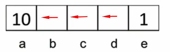
Q2: For Y = 0.1:
-
If I'm at state
a, I will exit and get reward of 10. -
If I'm at state
b, I will move left because the sum of discounted rewards is 1 (0+0.1 * 10). If I move right, the sum of discounted rewards is 0.001 (0.1^0*1). -
If I'm at state
c, I will move left because the sum of rewards is 0.1 (0+0.1*0+0.1^2 * 10). If I move right, the sum of rewards is 0.001 (0+0.1 * 0+0.1^2 * 0+0.1^3 * 10). -
If I'm at state
d, I will moverightbecause the sum of rewards is 0.1 (0+0.1). If I move left, the sum of rewards is 0.001 (0+0.1 * 0+0.1^2 * 0+0.1^3 * 10).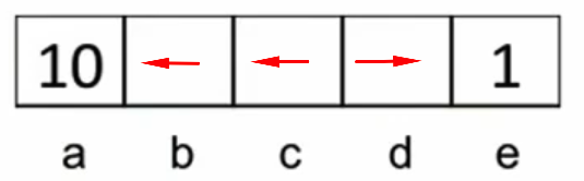
Q3: Solving the linear equation 0Y+ 0Y^2 + 10Y^3 = 1*Y, we get Y = 0.316.
Summary:
- Markov Decision Processes (MDPs) provide a mathematical framework for modeling decision making in situations where outcomes are partly random and partly under the control of a decision maker.
- The word "Markov" in MDP refers to the fact that the future can be determined only from the present state (i.e., the future is independent of the past).
- A Markov decision process formalism consists of the following elements: a set of states S, a set of actions A, a reward function R, and a transition probability model P.
- The goal of the Markov Decision Process is to find a good policy π for the decision maker. A policy is a function that maps states to actions (π: S → A). The policy tells the agent what action to take in each state. The goal is to find the policy that maximizes the expected total reward.
- The optimal policy is the policy that maximizes the expected total reward. The optimal policy is denoted by π*.
- The discount factor is a value between 0 and 1 and it decays after each step. It is used to model the fact that the future rewards are worth less than its value due to the delay in receiving them.