Course Overview
Welcome to CSE005 , Artificial Intelligence (AI). You are joining a global learning community dedicated to helping you learn and thrive in the AI era.
📺 Watch this welcome video from your instructor.
Course Description
Artificial Intelligence (AI) aims to teach students the techniques for building computer systems that exhibit intelligent behavior. AI is one of the most consequential applications of computer science, and is helping to solve complex real-world problems, from self-driving cars to facial recognition. This course will teach students the theory and techniques of AI, so that they understand how AI methods work under a variety of conditions.
The course begins with an exploration of the historical development of AI, and helps students understand the key problems that are studied and the key ideas that have emerged from research. Then, students learn a set of methods that cover: problem solving, search algorithms, knowledge representation and reasoning, natural language understanding, and computer vision. Throughout the course, as they apply technical methods, students will also examine pressing ethical concerns that are resulting from AI, including privacy and surveillance, transparency, bias, and more.
Course assignments will consist of short programming exercises and discussion-oriented readings. The course culminates in a final group project and accompanying paper that allows students to apply concepts to a problem of personal interest.
Topics
- Intelligent Agents
- Search strategies
- Game Playing
- Knowledge and Reasoning
- Natural Language Processing
- Computer Vision
- Ethics and safety
How the course works
There are multiple ways you'll learn in this course:
- Read and engage with the materials on this site
- Attend live class and complete the activities in class
- Answer practice exercises to try out the concepts
- Complete assignments and projects to demonstrate what you have learned
Active engagement is necessary for success in the course! You should try to write lots of programs, so that you can explore the concepts in a variety of ways.
You are encouraged to seek out additional practice problems outside of the practice problems included in the course.
Learning Outcomes
By the end of the course, students will be able to:
- Demonstrate understanding of the foundation and history of AI
- Explain basic knowledge representation, problem solving, inference, and learning methods of AI
- Develop intelligent systems to solve real-world problems by selecting and applying appropriate algorithms
- Explain the capabilities and limitations of various AI algorithms and techniques
- Participate meaningfully in discussions of AI, including its current scope and limitations, and societal implications
Instructor
- Mohammed Saudi
- mohammed.saudi@kibo.school
Please contact on Discord first with questions about the course.
Live Class Time
Note: all times are shown in GMT.
- Wednesday, 15:00 - 16:30 GMT
Office Hours
- Tuesday, 15:00 - 16:30 GMT
Core Reading List
- Norvig P., Russell S. (2020). Artificial Intelligence: A Modern Approach. Pearson, 4th e. (Chapters 1-12, 23, 24, 25,27)
Supplemental Reading List
- Zhang A, Lipton Zn, Li M, Smola A. (2021) Dive into Deep Learning
Live Classes
Each week, you will have a live class (see course overview for time). You are required to attend the live class sessions.
Video recordings and resources for the class will be posted after the classes each week. If you have technical difficulties or are occasionally unable to attend the live class, please be sure to watch the recording as quickly as possible so that you do not fall behind.
Live Classes Feedback Form: Feedback Form
| Week | Topic | Live Class | Slides | Code |
|---|---|---|---|---|
| 1 | Intelligence Via Search | video | slides | code |
| 2 | Game Playing | video | slides | |
| 3 | CSPs | video | slides | code |
| 4 | Reinforcement Learning | video | slides | code |
| 5 | Supervised Learning | video | slides | code |
| 6 | CNN | video | slides | code 1 code 2 |
| 7 | Logic | video | slides | code 1 code 2 |
| 8 | NLP | video | slides | code |
Assessments & Grading
In this course, you will be assessed on your ability to apply the concepts and techniques covered in class to solve problems. You will be assessed through a combination of programming assignments, quizzes, and a final project.
You overall course grade is composed of these weighted elements:
- Programming Assignments & Oral Exams: 40%
- Quizzes: 40%
- Final Project: 20%
Programming Assignments
Each week, you will be given a programming assignment to complete. These assignments will be graded based on the correctness of your solution, as well as the quality of your code. You will be expected to submit your code on GitHub, and your code will be reviewed by the instructor.
Late Policy
Please review the late submission policy for each assignment on the assignment details page.
Quizzes
There will be weekly quizzes to test your understanding of the material. These quizzes will be a combination of multiple choice, short answer, and programming questions. You will be expected to complete these quizzes on your own, without any external help.
Oral Exams
Based on your coursework and assignment submissions, you may be required to participate in an oral exam. This is designed to ensure that you have a solid understanding of the course material and have independently completed your work.
Final Project/Exam
A final project will be submitted by the end of the term. You will have the last two weeks to complete it. More details will be provided later.
Getting Help
If you have any trouble understanding the concepts or stuck on a problem, we expect you to reach out for help!
Below are the different ways to get help in this class.
Discord Channel
The first place to go is always the course's help channel on Discord. Share your question there so that your Instructor and your peers can help as soon as we can. Peers should jump in and help answer questions (see the Getting and Giving Help sections for some guidelines).
Message your Instructor on Discord
If your question doesn't get resolved within 24 hours on Discord, you can reach out to your instructor directly via Discord DM or Email.
Office Hours
There will be weekly office hours with your Instructor and your TA. Please make use of them!
Tips on Asking Good Questions
Asking effective questions is a crucial skill for any computer science student. Here are some guidelines to help structure questions effectively:
-
Be Specific:
- Clearly state the problem or concept you're struggling with.
- Avoid vague or broad questions. The more specific you are, the easier it is for others to help.
-
Provide Context:
- Include relevant details about your environment, programming language, tools, and any error messages you're encountering.
- Explain what you're trying to achieve and any steps you've already taken to solve the problem.
-
Show Your Work:
- If your question involves code, provide a minimal, complete, verifiable, and reproducible example (a "MCVE") that demonstrates the issue.
- Highlight the specific lines or sections where you believe the problem lies.
-
Highlight Error Messages:
- If you're getting error messages, include them in your question. Understanding the error is often crucial to finding a solution.
-
Research First:
- Demonstrate that you've made an effort to solve the problem on your own. Share what you've found in your research and explain why it didn't fully solve your issue.
-
Use Clear Language:
- Clearly articulate your question. Avoid jargon or overly technical terms if you're unsure of their meaning.
- Proofread your question to ensure it's grammatically correct and easy to understand.
-
Be Patient and Respectful:
- Be patient while waiting for a response.
- Show gratitude when someone helps you, and be open to feedback.
-
Ask for Understanding, Not Just Solutions:
- Instead of just asking for the solution, try to understand the underlying concepts. This will help you learn and become more self-sufficient in problem-solving.
-
Provide Updates:
- If you make progress or find a solution on your own, share it with those who are helping you. It not only shows gratitude but also helps others who might have a similar issue.
Remember, effective communication is key to getting the help you need both in school and professionally. Following these guidelines will not only help you in receiving quality assistance but will also contribute to a positive and collaborative community experience.
Screenshots
It’s often helpful to include a screenshot with your question. Here’s how:
- Windows: press the Windows key + Print Screen key
- the screenshot will be saved to the Pictures > Screenshots folder
- alternatively: press the Windows key + Shift + S to open the snipping tool
- Mac: press the Command key + Shift key + 4
- it will save to your desktop, and show as a thumbnail
Giving Help
Providing help to peers in a way that fosters learning and collaboration while maintaining academic integrity is crucial. Here are some guidelines that a computer science university student can follow:
-
Understand University Policies:
- Familiarize yourself with Kibo's Academic Honesty and Integrity Policy. This policy is designed to protect the value of your degree, which is ultimately determined by the ability of our graduates to apply their knowledge and skills to develop high quality solutions to challenging problems--not their grades!
-
Encourage Independent Learning:
- Rather than giving direct answers, guide your peers to resources, references, or methodologies that can help them solve the problem on their own. Encourage them to understand the concepts rather than just finding the correct solution. Work through examples that are different from the assignments or practice problems provide in the course to demonstrate the concepts.
-
Collaborate, Don't Complete:
- Collaborate on ideas and concepts, but avoid completing assignments or projects for others. Provide suggestions, share insights, and discuss approaches without doing the work for them or showing your work to them.
-
Set Boundaries:
- Make it clear that you're willing to help with understanding concepts and problem-solving, but you won't assist in any activity that violates academic integrity policies.
-
Use Group Study Sessions:
- Participate in group study sessions where everyone can contribute and learn together. This way, ideas are shared, but each individual is responsible for their own understanding and work.
-
Be Mindful of Collaboration Tools:
- If using collaboration tools like version control systems or shared documents, make sure that contributions are clear and well-documented. Clearly delineate individual contributions to avoid confusion.
-
Refer to Resources:
- Direct your peers to relevant textbooks, online resources, or documentation. Learning to find and use resources is an essential skill, and guiding them toward these materials can be immensely helpful both in the moment and your career.
-
Ask Probing Questions:
- Instead of providing direct answers, ask questions that guide your peers to think critically about the problem. This helps them develop problem-solving skills.
-
Be Transparent:
- If you're unsure about the appropriateness of your assistance, it's better to seek guidance from professors or teaching assistants. Be transparent about the level of help you're providing.
-
Promote Honesty:
- Encourage your peers to take pride in their work and to be honest about the level of help they received. Acknowledging assistance is a key aspect of academic integrity.
Remember, the goal is to create an environment where students can learn from each other (after all, we are better together) while we develop our individual skills and understanding of the subject matter.
Academic Integrity
When you turn in any work that is graded, you are representing that the work is your own. Copying work from another student or from an online resource and submitting it is plagiarism. Using generative AI tools such as ChatGPT to help you understand concepts (i.e., as though it is your own personal tutor) is valuable. However, you should not submit work generated by these tools as though it is your own work. Remember, the activities we assign are your opportunity to prove to yourself (and to us) that you understand the concepts. Using these tools to generate answers to assignments may help you in the short-term, but not in the long-term.
As a reminder of Kibo's academic honesty and integrity policy: Any student found to be committing academic misconduct will be subject to disciplinary action including dismissal.
Disciplinary action may include:
- Failing the assignment
- Failing the course
- Dismissal from Kibo
For more information about what counts as plagiarism and tips for working with integrity, review the "What is Plagiarism?" Video and Slides.
The full Kibo policy on Academic Honesty and Integrity Policy is available here.
Course Tools
In this course, we are using these tools to work on code. If you haven't set up your laptop and installed the software yet, follow the guide in https://github.com/kiboschool/setup-guides.
- GitHub is a website that hosts code. We'll use it as a place to keep our project and assignment code.
- GitHub Classroom is a tool for assigning individual and team projects on Github.
- Visual Studio Code is an Integrated Development Environment (IDE) that has many plugins which can extend the features and capabilities of the application. Take time to learn how ot use VS Code (and other key tools) because you will ultimately save enormous amounts of time.
- Anchor is Kibo's Learning Management System (LMS). You will access your course content through this website, track your progress, and see your grades through this site.
- Gradescope is a grading platform. We'll use it to track assignment submissions and give you feedback on your work.
- Woolf is our accreditation partner. We'll track work there too, so that you get credit towards your degree.
Intelligence via Search

You will acquire practical skills in modeling and constructing programs to achieve intelligence by addressing search problems. We will learn how to solve problems such as maze navigation and pathfinding using various search algorithms like depth-first search, breadth-first search, and A* search.
This Week's Work:
- Study the material and complete the practical exercises.
- Complete the quiz and coding assignment for this week. The coding assignment will involve building a shipping route planner using the A* search algorithm.
Upon completing this week's work, you will be able to:
- Develop intelligent software agents capable of solving diverse problems, such as pathfinding and playing games like the 15-puzzle.
- Explain the field of AI and its fundamental concepts.
AI: What and Why

Intelligence
If a robot navigates city streets without colliding with anything, would you consider this robot intelligent? Many would agree, myself included. However, if a human performs the same task, you might hesitate to describe them as intelligent. On the other hand, when a person tackles a challenging math problem or quickly learns a new language, we are more inclined to label them as intelligent.
Some have seen intelligence as the ability to use language, form abstractions and concepts, solve problems, and acquire knowledge.Turing Test
In the 1950s, Alan Turing, a British computer scientist, proposed a test to determine whether a machine can think. The test, known as the Turing test, involves a human evaluator who engages in a natural language conversation with two other parties: one human and one machine. If the evaluator cannot distinguish between the human and the machine, the machine is considered intelligent. This test is still used today to assess the intelligence of machines.
(Optional) Watch the video below to learn more about the Turing test:
Defining Intelligence
A widely accepted definition of intelligence is the ability to make the correct decisions. But what does it mean to make the correct decision? To answer this question, we need to delve into the concept of rationality.
Rationality
From a scientific standpoint, rationality is the quality of being grounded in reason and logic. Thus, a person or a machine is considered rational if their decisions are based on reasoning and logic, and are guided by specific goals.

Example of Rationality:
Suppose we have an agent (software, a person, or a machine) playing chess. In this context, making the move expected to maximize the chances of winning the game is the right decision. This exemplifies rationality because the agent is making a decision based on reasoning and logic, aimed at achieving a specific goal: winning the game.
Another example of rationality:
Imagine an agent operating a vehicle. Here, making choices aimed at maximizing the likelihood of reaching the destination safely, and perhaps quickly, represents the right course of action. This too embodies rationality, with decisions derived from reasoning and logic in pursuit of the specific goal of arriving safely and efficiently.
Human agents rely on sensory organs like eyes and ears, along with limbs such as hands and legs, to perceive and interact with their surroundings. In contrast, robotic agents are equipped with specialized sensors like cameras and infrared range finders, enabling them to sense their environment, while actuators such as motors enable them to move and manipulate objects.
Software agents, on the other hand, interpret inputs such as keystrokes, file contents, and network packets, using them to execute tasks like displaying information on a screen, storing data in files, or transmitting data over networks.
Artificial Intelligence (AI)
Artificial Intelligence (AI) is the field of building systems that can think and act rationally.
AI is about building computer systems that can replicate various human activities, such as walking, seeing, understanding, speaking, learning, responding, and many others.
The AI dream is to someday build machines as intelligent as humans (capable of doing multiple tasks intelligently). This is sometimes called Artificial General Intelligence or AGI.
Machine Learning
Machine learning, a subfield of AI, focuses on building systems that can learn from data or, in other words, make rational decisions based on data.
Deep Learning
Deep learning is a subset of machine learning that centers on developing machines capable of learning from data using deep neural networks.
In future lessons, we will discuss machine learning and deep learning in more detail.
Why AI Now?
The history of AI dates back to the 1950s. If you'd like a quick three-minute recap of AI's history, you can watch this video:
The question we want to address here is why AI is currently experiencing a surge in attention. There are several significant factors contributing to this phenomenon; I will highlight the two most important ones:
Data
The availability of extensive public datasets has profoundly transformed the AI landscape. These datasets, often curated and made accessible by organizations, government agencies, or academic collaborations, provide copious amounts of diverse, well-structured, and labeled data. Prominent examples include ImageNet for image recognition, the Common Crawl for natural language processing, and the Human Genome Project for genomics. Access to such extensive public datasets has enabled AI researchers to train their models on data that represents a broader spectrum of real-world scenarios, leading to substantial improvements in AI system performance and accuracy.
Hardware
Advancements in hardware technology, especially the development of high-performance graphics processing units (GPUs) and specialized AI accelerators like TPUs (Tensor Processing Units), have significantly increased the computational power available for AI tasks. AI models, particularly deep learning neural networks, demand substantial computational resources for training and inference. The enhancement in computational capabilities has empowered researchers to work with more extensive and complex models, resulting in improved AI performance.
Although GPUs and TPUs can be costly to purchase and operate, they are now widely accessible in the cloud, making them affordable for a broader audience. This accessibility has facilitated AI researchers and practitioners in experimenting with more intricate models and larger datasets without requiring substantial investments in expensive hardware.
Here is a screenshot of the Google Cloud Platform which provides access to GPUs and TPUs:

Summary:
-
AI is the field of building systems that can think and act rationally (guided by reasoning, logic, knowledge, and specific goals).
-
The term "agent" is used to describe an entity striving to achieve specific objectives. An agent can be a person, a machine, software, or a combination of these.
-
AI is getting so much attention now due to many reasons including the availability of large public datasets and the advancement of hardware technologies.
Check your understanding:
- Explain AI to a 10-year-old.
- List two reasons for the current surge of interest in AI.
Explore, Share, and Discuss:
Search the web and find some of the latest hardware devices that empower AI applications.
💬 Share your findings with us on Discord here.
Applications of AI in the Real World
Artificial Intelligence (AI) has become an integral part of our daily lives, revolutionizing various industries and solving complex problems. Below are just a few examples of AI applications in the real world.
Healthcare:
-
Medical Imaging: AI is used to analyze medical images such as X-rays, MRIs, and CT scans, helping detect diseases, tumors, and anomalies. For example, Google's DeepMind developed an AI system capable of diagnosing eye diseases like diabetic retinopathy from retinal scans.
-
Drug Discovery: AI accelerates drug discovery by predicting potential drug candidates and simulating their effects. Companies like Atomwise use AI to discover new medicines for various diseases, reducing research time.
Finance:
-
Algorithmic Trading: AI is employed to make high-frequency trades, analyze market data, and make split-second decisions. Companies like Renaissance Technologies use AI for hedge fund management.
-
Fraud Detection: Banks and financial institutions use AI to detect fraudulent activities. For instance, PayPal employs AI to spot suspicious transactions and prevent fraud.
Transportation:
-
Self-Driving Cars: Companies like Tesla, Waymo, and Uber are developing self-driving cars that use AI for real-time navigation and collision avoidance.
-
Traffic Management: AI optimizes traffic flow, reduces congestion, and enhances public transportation. Cities like Singapore use AI for traffic light control, reducing travel times.
Education:
-
Personalized Learning: AI-powered educational platforms like Duolingo adapt to individual learning styles and provide personalized learning paths.
-
Plagiarism Detection: AI systems, such as Turnitin, scan student papers and detect instances of plagiarism.
Retail:
-
Recommendation Systems: E-commerce giants like Amazon use AI to recommend products to customers based on their browsing and purchase history.
-
Inventory Management: AI optimizes inventory levels, reducing costs and minimizing waste. Walmart uses AI for demand forecasting and stock replenishment.
Entertainment:
-
Content Recommendation: Streaming services like Netflix and Spotify use AI to suggest movies, shows, and music based on user preferences.
-
Content Creation: AI is used to generate content, such as deepfake videos and AI-written articles, but it also has potential for creative content generation in the future.
Agriculture:
-
Precision Agriculture: AI-driven drones and sensors are used to monitor crops, soil quality, and weather conditions. This helps farmers make informed decisions about irrigation, fertilization, and pest control.
-
Crop Disease Detection: AI systems can identify crop diseases from images, enabling early intervention to save crops. AgShift, for example, uses AI to identify defects in harvested fruits.
Security:
-
Facial Recognition: AI is employed in security systems to identify individuals at airports, in public spaces, and on smartphones.
-
Cybersecurity: AI is used to detect and prevent cyber threats by analyzing patterns of malicious activities. Companies like Darktrace employ AI for real-time threat detection.
Think, Share and Discuss:
Think of a use case that you haven't seen in this lesson and try to explain how AI can be used to solve it. The highest voted answer will be featured in the next lesson.
💬 Share it with us on Discord here.
Search Problem Modeling
Ready for some excitement?
Would you be interested in learning how to program a computer to solve mazes, puzzles, find paths, or optimize item arrangements? What if you could also use this knowledge to minimize your time spent in traffic or create a system that plays chess or solves a Rubik's cube? This is precisely the essence of our lesson on "Search."

Search Problems
A search problem is a specific type of computational problem that involves exploring a set of possible states or configurations (known as the state space) and finding a sequence of actions to achieve a goal within this state space.
This is a broad definition, so let's clarify it with an example.
Consider the scenario of a car moving from point A to point B, as illustrated below:
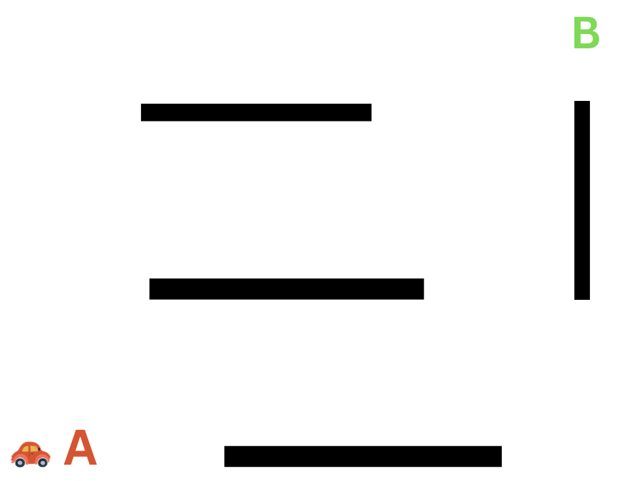
To reach point B, the car can follow various paths, as shown in the image below:
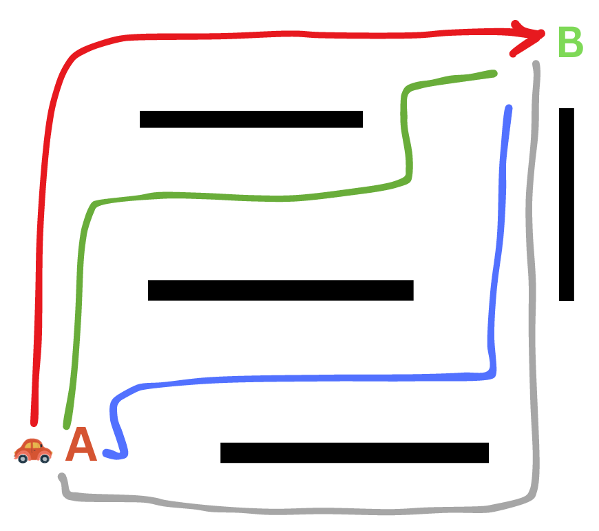
This is a search problem identified by the following:
- We have an agent (the car) that is trying to find a solution (the path) within a defined problem space (the road).
- The agent in this case is called a problem-solving agent.
- The problem space, or state space, consists of various states or configurations (the different positions of the car).
- The goal is to find a sequence of actions that will lead from an initial state (the starting position of the car) to a desired goal state (the destination).
The 8 Queens Problem
Let's consider another example. If we have a chessboard and eight queens, how can we place the queens on the chessboard so that no queen can attack another queen? This is known as the 8 queens problem.
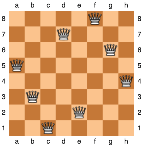
This is also a search problem identified by the following:
- There are various configurations (states) of the queens on the chessboard.
- The goal is to find a sequence of actions that will lead from an initial state (empty board) to a desired goal state (the configuration of the queens on the chessboard so that no queen can attack another queen).
More Examples
Here are a few more examples of search problems:
- Finding the optimal path for data packets to travel from a source to a destination
- Solving puzzles like Sudoku or Rubik's Cube
- Determining the optimal route between two locations on a map
You will learn how to solve such problems in this course 🚀.
🎯 Understanding Our Objective
One might question whether we are genuinely searching for something in this context. Well, you can think of the solution itself as the object of our search.
The solution is the sequence of actions that will lead us from the initial state to the goal state.
In the car example, our mission is to discover the path leading us to point B (by searching possible states). In the 8-queens problem, our mission is to find the configuration of the queens on the chessboard (by searching possible states starting with an initial one).
Modeling Search Problems
To tackle these problems with a computer, we aim to create a computer-friendly representation, a computational model. A typical model of a search problem consists of the following:
State Space:
This represents the different configurations of the problem space. For instance, the different positions of the car, the different arrangements of tiles in a puzzle, or the different configurations of a robot.
Initial State:
The starting state of the problem. For example, the starting position of the car, the initial arrangement of tiles in a puzzle, the initial position of a robot, etc.
Goal State:
The desired state of the problem. For example, it could be the car's destination, the desired puzzle tile arrangement, or the robot's target position. A goal test is a function that determines whether a given state is a goal state. For instance, checking if the car has reached its destination, if the puzzle tiles are in the correct order, or if the robot has arrived at its destination.
Actions:
Actions are the possible moves or steps that can transition the system from one state to another. These can include actions like moving up, down, left, or right.
Transition Model:
The transition model (or Successor Function) is a function that accepts a state and an action as input and yields an allowable new state as output. For example, the transition model for the car problem would take the car's current position and the desired direction, Up for example, as input and return the new position as output.
Solution:
The solution is a series of actions that lead from the initial state to the goal state. This could be the path the car takes from its starting point to its destination, the sequence of moves needed to solve the puzzle, or the route the robot follows to reach its goal.
Modeling the Car's Journey
Let's explore our previous example of a car journeying from point A to point B and frame it as a search problem. Our focus in this lesson is on modeling the problem's state space, initial state, goal state, goal test, actions, and transition model. The solution will be discussed in an upcoming lesson.
State Space:
To model the state space, we need to consider all the possible configurations of the car. To do that, we need to decide how we will represent the car's position and the environment in which it is moving.
To simplify things, we can represent the car's position as a coordinate on a grid. For example, the car's position at point A can be represented as (1,0), and its position at point B can be represented as (6,6).
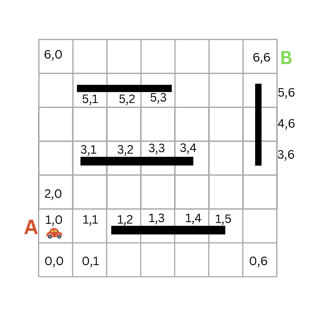
So, the state space is all the possible positions of the car on the grid. This is a finite set of states, and we can represent it as a list in Python.
state_space = []
GRID_SIZE = 6
for i in range(GRID_SIZE):
    for j in range(GRID_SIZE):
        state_space.append(1)
Important Note: The state space in this example is small enough to be represented as a list. However, in most cases, the state space is too large to be represented as a list, as in this example, and we don't need to store the entire state space upfront. More information on this will be provided later.
Initial State:
After modeling the state space, it is clear now that our initial state is the position of the car at point A, which is (1, 0). We can represent the initial state as a tuple in Python.
initial_state = (1, 0)
Goal State and Goal Test:
The goal state is the position of the car at point B, which is (6, 6). Similarly, We can represent the goal state as a tuple in Python.
goal_state = (6, 6)
The goal test will be a function that checks if the car's current position is the same as the goal position. If so, it returns True; otherwise, it returns False.
def goal_test(state):
    return state == goal_state
Actions:
Actions are the possible moves or steps that can transition the system from one state to another. In our example, the car can move up, down, left, or right. We can represent the actions as a list in Python.
actions = ["up", "down", "left", "right"]
Transition Model (Successor Function)
At a specific state, the agent can take one of the possible actions: up, down, left, or right. For each specific action, the agent will end up in a new state.
Try it!
Take 10 minutes and try to write a transition model function for our car example. It's a function that should take a state and an action as input and return a new state as output.
def transition_model(state, action):
    # Your code here
Recall that the current state is the position of the car within the grid. The action is the direction the car is moving in. For example, if the car is at position (1, 1) and the action is up, the newly returned position will be (2, 1).
Don't rush through it. This is a crucial step in your learning process. If you can't do it, you can check the solution below. But, please, try to do it first.

Unfold the sample code below for an idea of how a transition model for this environment can be implemented.
Transition Model Function
def transition_model(state, action):
    x, y = state
    if action == 'up':
        return (x, y + 1)
    elif action == 'down':
        return (x, y - 1)
    elif action == 'left':
        return (x - 1, y)
    elif action == 'right':
        return (x + 1, y)
    else:
        raise ValueError(f"Unknown action: {action}")
- Note: The sample code above does not check if the new state is valid or not.
Exercise: The 8-Puzzle Problem
Now, it's your turn to model a search problem.
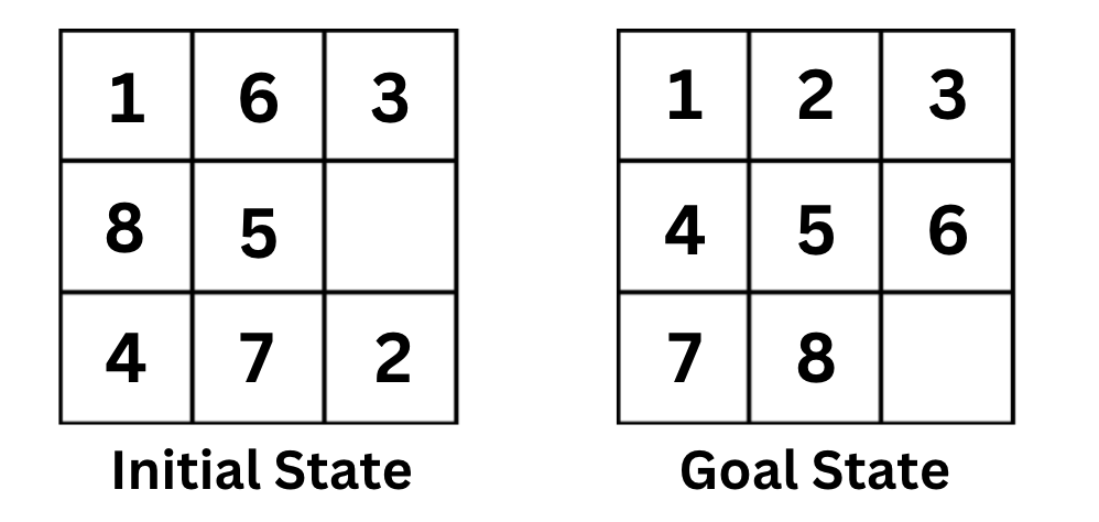
The 8-puzzle was invented and popularized by Noyes Palmer Chapman in the 1870s. It is played on a 3-by-3 grid with 8 square blocks labeled 1 through 8 and a blank square. Your goal is to rearrange the blocks so that they are in order. You are permitted to slide blocks horizontally or vertically into the blank square.
Take 10-15 minutes and try to model this problem. Describe the state space, initial state, goal test, actions, and transition model.
This is a crucial step in your learning process. Don't rush through it.

🧩 Unfold the solution below and match it with your solution.
Solution
State Space: The state space is all the possible configurations of the puzzle tiles. [[1, 3, 2], [6, 4, 7], [7, 8, None]] and [3, 1, 2], [6, 4, 7], [8, 7, None]] are two examples of states in the state space.
Initial State: The initial state is the starting configuration of the puzzle, which may initially be a scrambled arrangement of the tiles. For example, [[1, 3, 2], [6, 4, 7], [7, 8, None]].
Goal State: The goal state is the desired configuration where the tiles are arranged in ascending order [[1, 2, 3], [4, 5, 6], [7, 8, None]]. The Goal Test is a function that checks if the current state is the goal state.
Actions: Moving the blank tile up, down, left, or right.
Transition Model: This function defines the outcome of applying an action to a given state, resulting in a new state. For example, if the current state is [[1, 6, 3], [8, None, 5], [4, 7, 2]] and the action is up, the new state will be [[1, 6, 3], [8, 7, 5], [4, None, 2]]
![]()
🎉 Congratulations!🎉
You have just completed modeling your first search problem!
State and State Space Representation
In any search problem, the method of representing states and state space significantly influences the efficiency of our search algorithms.
For example, in the car navigation problem, rather than using a tuple representation, we can opt for a graph representation. In this scenario, nodes symbolize specific car configurations, while edges illustrate permissible movements between them.
Likewise, in the 8-puzzle problem, a graph representation is applicable, where each node denotes a specific puzzle configuration, and the edges represent the feasible transitions between configurations.
Choosing a graph representation may provide the flexibility to utilize various graph algorithms, potentially optimizing the search process and improving problem-solving efficiency.
This concept can be expanded further by incorporating additional information into the representation, such as the estimated cost of reaching the goal from a particular state, to guide the search process and enhance the search algorithms' efficiency.
💡 Exploring different methods for representing states and state spaces is an interesting area of research. You could be the next person to devise an innovative representation of states and state spaces for a specific problem, thereby making your mark as a computer scientist in the field.
Can you think of other ways to represent states and state spaces for any of the problems discussed in this lesson?
💬 Discuss and share your thoughts with us here.
Self Assessment!
-
What is a search problem?
-
What are the components of a search problem?
-
Give a complete problem formulation for each of the following problems. Choose a formulation that is precise enough to be implemented.
-
There is an n×n grid of squares, each square initially being either an unpainted floor or a bottomless pit. You start standing on an unpainted floor square and can either paint the square under you or move onto an adjacent unpainted floor square. You want the whole floor painted.
-
Your goal is to navigate a robot out of a maze. The robot starts in the center of the maze facing north. You can turn the robot to face north, east, south, or west. You can direct the robot to move forward a certain distance, although it will stop before hitting a wall.
-
Unfold the sample solutions below to check your answers.
Sample Solutions
1. n×n grid of squares
State space: all possible configurations of the floor tiles and your position.
Initial state: all floor squares unpainted, you start standing on one square unpainted floor square. Actions: paint square, move to adjacent floor square.
Goal test: all floor squares painted.
Successor function: paint current tile, move to adjacent unpainted floor tile.
2. navigate a robot out of a maze
We’ll define the coordinate system so that the center of the maze is at (0, 0), and the maze itself is a square from (−1, −1) to (1, 1).
State space: all possible locations and directions of the robot.
Initial state: robot at coordinate (0, 0), facing North.
Actions: turn north, turn south, turn east, turn west, move forward.
Goal test: either |x| > 1 or |y| > 1 where (x, y) is the current location.
Successor function: move forwards any distance d; change direction robot it facing. Cost function: total distance moved.
The output of the program is:
A* Solution:
# some steps omitted
.....
Move up:
[1, 2, 3, 4]
[5, 6, 11, 7]
[9, 10, 0, 8]
[13, 14, 15, 12]


Move up:
[1, 2, 3, 4]
[5, 6, 0, 7]
[9, 10, 11, 8]
[13, 14, 15, 12]


Move right:
[1, 2, 3, 4]
[5, 6, 7, 0]
[9, 10, 11, 8]
[13, 14, 15, 12]


Move down:
[1, 2, 3, 4]
[5, 6, 7, 8]
[9, 10, 11, 0]
[13, 14, 15, 12]


Move down:
[1, 2, 3, 4]
[5, 6, 7, 8]
[9, 10, 11, 12]
[13, 14, 15, 0]

24
Comparing that with the number of steps taken by the greedy best-first search algorithm, we can see that the A* search algorithm found the optimal solution with 24 steps, while the greedy best-first search algorithm found a solution with 187 steps.
Variants of A* Search
A* (A-star) search is a widely used algorithm for finding the shortest path in a graph or solving optimization problems. It uses a heuristic to guide the search, making it more efficient than traditional uninformed search algorithms. There are different variations of A* search, each tailored to specific types of problems or computational constraints. Here are some notable variations:
Basic A* Search:
The standard A algorithm uses a combination of the cost to reach a node (g) and a heuristic estimate of the cost to reach the goal from that node (h). The evaluation function is f(n) = g(n) + h(n). A expands nodes with the lowest f(n) value.
Weighted A* Search:
Weighted A* introduces a weight factor to the heuristic function, influencing the balance between the cost to reach the node and the estimated cost to the goal. This can be useful for adjusting the algorithm's behavior, favoring either optimality or speed.
Bidirectional A* Search:
In bidirectional A* search, the search is performed simultaneously from both the start and goal states. The algorithm continues until the two searches meet in the middle. This approach can be more efficient for certain types of graphs, especially when the branching factor is high.
Real-Time A* Search:
Real-Time A* is an extension of A* designed for environments where computation time is limited. It uses an incremental approach, exploring nodes in the order of their estimated cost until the available time runs out, returning the best solution found.
These variations address different challenges and requirements, making A* adaptable to a wide range of problem domains and computational constraints. The choice of a specific variation depends on the characteristics of the problem, available resources, and the desired trade-offs between optimality and efficiency.
Summary
The A* search algorithm is an informed search algorithm that uses both the cost of the path and the heuristic function to guide its search. The A* search algorithm is guaranteed to find the optimal solution if the heuristic function is admissible and consistent.
More Heuristics
As discussed in our previous lessons, various heuristic functions can guide the search. We used the number of misplaced tiles as our heuristic function in the 15-puzzle example and the Manhattan distance in our car example. Here are a few more common heuristics with sample implementations for you to explore.
Euclidean Distance
The Euclidean distance is the straight-line distance between two points in Euclidean space. It is named after the ancient Greek mathematician Euclid, who introduced the concept of Euclidean space.
def euclidean_distance(board, goal_board):
  distance = 0
  for i in range(N * N):
    if board[i] != 0:  # Skip the empty tile
      correct_pos = goal_board.index(board[i])
      current_row, current_col = divmod(i, N)
      correct_row, correct_col = divmod(correct_pos, N)
      distance += math.sqrt((current_row - correct_row)**2 +
                            (current_col - correct_col)**2)
  return distance
Hamming Distance
The Hamming distance is the number of positions at which two strings of equal length differ. It is named after the American mathematician Richard Hamming.
def hamming_distance(board, goal_board):
  distance = 0
  for i in range(N * N):
    if board[i] != 0 and board[i] != goal_board[i]:
      distance += 1
  return distance
Manhattan Distance
The Manhattan distance is the sum of the horizontal and vertical distances between two points on a grid. It is named after the grid-like layout of the streets in Manhattan.
def manhattan_distance(board, goal_board):
  distance = 0
  for i in range(N * N):
    if board[i] != 0:  # Skip the empty tile
      correct_pos = goal_board.index(board[i])
      current_row, current_col = divmod(i, N)
      correct_row, correct_col = divmod(correct_pos, N)
      distance += abs(current_row - correct_row) + abs(current_col -
                                                       correct_col)
  return distance
Linear Conflict
The linear conflict heuristic is a modification of the Manhattan distance heuristic. It is calculated by adding the number of moves required to resolve each linear conflict to the Manhattan distance.
A linear conflict occurs when two tiles are in their goal row or column, but are reversed relative to their goal positions. For example, if the tile 1 is in the second row and the tile 2 is in the first row, then they are in a linear conflict. To resolve this conflict, we need to move one of the tiles out of the way, so that the other tile can move into its correct position. This requires two moves, one for each tile.
def linear_conflict(board, goal_board):
  conflict_count = 0
  for i in range(N * N):
    if board[i] != 0:  # Skip the empty tile
      correct_pos = goal_board.index(board[i])
      current_row, current_col = divmod(i, N)
      correct_row, correct_col = divmod(correct_pos, N)
      if current_row == correct_row and current_col == correct_col:
        continue
      if current_row == correct_row:
        for j in range(i + 1, N * N):
          if board[j] != 0 and goal_board.index(board[j]) < correct_pos:
            conflict_count += 1
      if current_col == correct_col:
        for j in range(i + N, N * N, N):
          if board[j] != 0 and goal_board.index(board[j]) < correct_pos:
            conflict_count += 1
  return conflict_count * 2
Online N-Puzzle Solver
Here is a cool online repository that solves the 15-puzzle problem using various algorithms and heuristics.

Summary
Heuristic functions are used to guide the search algorithm to find the optimal solution faster. A heuristic function is admissible if it never overestimates the cost of reaching the goal, and it is consistent if the estimated cost of reaching the goal from node n is less than or equal to the cost of reaching node n' from node n plus the estimated cost of reaching the goal from node n'.
Different problems require different heuristic functions. The design of an effective heuristic function is a challenging task and requires a good understanding of the problem. It significantly affects the performance of the search algorithm.
Quiz 1: Intelligence via Search
Before attempting the quiz, read the following carefully.
- This is a timed quiz. You will have only one attempt.
- You will have 40 minutes to complete multiple-choice questions.
- You should first study the lesson materials thoroughly. More specifically, you should learn about search problems, search problem formulation, tracing and running search algorithms, and heuristic functions.
➡️ Access the quiz on Gradescope here.
Week 1 Assignment: Shipping Route Finder
In this assignment, you will implement a shipping route finder program that utilizes the A* search algorithm to determine the shortest path between two shipping points.
➡️ Access the assignment and all details here.
Intelligence via Search II
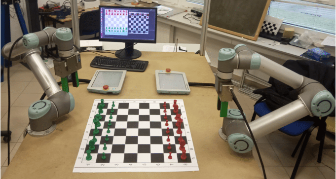
https://www.researchgate.net/figure/Collaborative-robot-system-for-playing-chess_fig4_345377838
Hello, and welcome to the second part of the "Intelligence via Search" lesson. In this lesson, we will continue to explore search algorithms and their applications in the field of artificial intelligence. More specifically, we will discuss game playing and how search algorithms can be used.
This Week's Work:
- Study the material and solve the practical exercises.
- Complete the quiz and coding assignment for this week.
- The coding assignment will involve building a tic-tac-toe game-playing agent using the minimax with alpha-beta pruning algorithm.
Upon completing this week's work, you will be able to:
- Explain the concept of game playing and its relevance to artificial intelligence.
- Describe the minimax algorithm and its application in game playing.
- Develop a game-playing agent capable of playing tic-tac-toe using the minimax algorithm.
Adversarial Search

So far, the problems we have examined have been single-agent problems. In other words, there is only one agent (such as a car or a player of a 15-puzzle game) attempting to solve the problem, such as finding a path to a goal point or rearranging the tiles to the correct order. However, in many problems, especially games, there are two agents trying to solve the problem, each one acting against the other. In this lesson, we will explore how to address such problems.
Adversarial Scenarios
In a pacman game, the pacman agent is trying to eat all the food pellets while avoiding the ghosts. The ghosts are trying to eat the pacman.
In a tic-tac-toe game, the two players are trying to get three of their pieces in a row before the other player does.
In trading, one trader is trying to buy low and sell high, while the other trader is trying to sell high and buy low.
These are all examples of adversarial scenarios. In each case, there are two agents trying to solve the same problem, but each one is acting against the other.
Solving Adversarial Search Problems
Let's dig deeper into how to solve adversarial search problems. Let's start with the tic-tac-toe game.
In a tic-tac-toe game like the one shown below, if you are the X player, what would be your next move and why?

I bet you chose to place X at position 5. Why? Because it is the move to prevent the O player from winning.


We know this because we are humans and we have played this game many times. But how can we teach a computer to play this game? Fortunately, scientists have come up with many strategies to solve it. One of these strategies is called the minimax algorithm. Let's explore it next.
Minimax Algorithm
The minimax algorithm is a strategy used in decision making, particularly in game theory and artificial intelligence, for minimizing the possible loss while maximizing the potential gain. It's often applied in two-player games like chess or tic-tac-toe. Here's how it works:
In a game, there are two players. One is the maximizer, who tries to get the highest score possible, while the other is the minimizer, who tries to do the opposite and minimize the score.
In a tic-tac-toe game, the maximizer for example is the player who has the X symbol and the minimizer is the player who has the O symbol. When X makes a move, it tries to maximize the score, while O tries to minimize it.
Considering the 3 possible outcomes of the game, X can either win, lose, or draw. If X wins, it gets a score of 1. If X loses, it gets a score of -1. If the game ends in a draw, both players get a score of 0.
To illustrate this, let's consider the game shown below.

It is player O's turn to make a move. O has two possible moves, either place O at position 1 or position 8. The algorithm will look ahead and examine the consequences of each possible move.
If O places its symbol at position 1, the player X will put its symbol at position 8, leading to a game score of 1 (X wins).
If O places its symbol at position 8, the player X will put its symbol at position 1 leading to a game score of 0 (tie).
Because O is a minimizer, it will choose the move that minimizes the score so the minimizer O will choose to place O at position 8.

Utility Values
The scores 1, 0, and -1 are called utility values. They are used to represent the outcome of a particular game state. A score of 1 typically indicates a win for the player whose turn it is to move. A score of 0 often represents a draw or a neutral outcome. A score of -1 usually denotes a loss for the player whose turn it is to move. You can use other numbers to represent the outcome of a game state. For example, you can use 10 to represent a win, 0 to represent a draw, and -10 to represent a loss but the convention is to use 1, 0, and -1.
Many Possible States
In an early stage of the game, there are many possible moves. Each move leads to a different game state. Before each move, the algorithm will look ahead and examine the consequences of each possible move. It will assume that the other player is also playing optimally. (trying to maximize its score). The algorithm will compute the score of each possible move and return the move with the highest score.

Recursive Algorithm
You might have guessed that the algorithm is recursive. It will keep looking ahead until it reaches a terminal state (a state where one of the players wins or the game is a tie).
Watch this video to learn more about the minimax algorithm.
Minimax Tree Traversal Exercise
In the below two-ply game tree:
-
Which move should the maximizer choose to maximize its score? 1 or 2?
-
What is the minimizer's best move if the maximizer chooses move 1? 3, 4, 5, or 6
-
What is the minimizer's best move if the maximizer chooses move 2? 7, 8, 9, or 10

Answer
-
We will first examine move #1. If the maximizer chooses move #1, the minimizer, in the following move, will choose between move #3,#4, #5, and #6 terminal states. Because the states are terminal, the algorithm will return the score of each one as given in the picture. Because the minimizer is trying to minimize the score, it will choose move #3 because it has a lower score of 99. Therfore, the score the maximizer will get if it chooses move #1 is 99.
-
Then we examine move #2. If the maximizer chooses move #2, the minimizer will choose between move #7, #8, #9, and #10. Because the minimizer is trying to minimize the score, it will choose move #7 or move #10 because they have the lowest score. Let's go with move #7. So the resulting score of move #2 is 100.
-
Between move #1 and move #2, the maximizer will choose move #2 because it has a higher score. Therefore, the score of move #1 is 100.

Minimax Pseudocode
function mini_max(state, is_maximizer_turn):
    if state is terminal
        return utility(state)
    if state is maximizer's turn
        max_value = -infinity
        for each action of available_actions(state)
            eval = mini_max(result(state,action)) # recursive call
            max_value = max(max_value, eval)
        return max_value
    if state is minimizer's turn
        min_value = +infinity
        for each action of available_actions(state)
            eval = mini_max(result(state,action)) # recursive call
            min_value = min(min_value, eval)
        return min_value
Here is a sample implementation in Python for the above minimax algorithm.
def minimax(board, is_maximizer_turn):
  # recursive terminal condition
  is_terminal = is_terminal_state(board)

  if is_terminal:
    return evaluate_utility(board)

  # else, keep expanding
  if is_maximizer_turn:
    best = float('-inf')
    for i in range(BOARD_SIZE):
      for j in range(BOARD_SIZE):
        if board[i][j] == EMPTY_CELL:  # the empty cell is a potential move
          board[i][j] = 'O'  # next player is 'O'
          score = minimax(board, not is_maximizer_turn) # it's the minimizer's turn
          best = max(best, score ) # get the max score of all possible moves
          board[i][j] = EMPTY_CELL # Undo the move to keep the board unchanged
    return best
  else:
    best = float('inf')
    for i in range(BOARD_SIZE):
      for j in range(BOARD_SIZE):
        if board[i][j] == EMPTY_CELL:  #the empty cell is a potential move
          board[i][j] = 'X'   #next player is 'X'
          score = minimax(board, not is_maximizer_turn)
          best = min(best, score) # get the minimum score of all possible moves
          board[i][j] = EMPTY_CELL
    return best
Tick-Tac-Toe AI
You may recall the below example of a tic-tac-toe game from your Programming 1 class.
print("Welcome to Tic-Tac-Toe")
print("Here is our playing board:")

# Constants
EMPTY_CELL = ' '
BOARD_SIZE = 3

# The play board
play_board = [[EMPTY_CELL for _ in range(BOARD_SIZE)]
              for _ in range(BOARD_SIZE)]


def evaluate_utility(board):
  # Checking for Rows for X or O victory.
  for row in range(BOARD_SIZE):
    if board[row][0] == board[row][1] == board[row][2]:
      if board[row][0] == 'O':
        return 1
      elif board[row][0] == 'X':
        return -1

  # Checking for Columns for X or O victory.
  for col in range(BOARD_SIZE):
    if board[0][col] == board[1][col] == board[2][col]:
      if board[0][col] == 'O':
        return 1
      elif board[0][col] == 'X':
        return -1

  # Checking for Diagonals for X or O victory.
  if board[0][0] == board[1][1] == board[2][2]:
    if board[0][0] == 'O':
      return 1
    elif board[0][0] == 'X':
      return -1

  if board[0][2] == board[1][1] == board[2][0]:
    if board[0][2] == 'O':
      return 1
    elif board[0][2] == 'X':
      return -1

  # Else if none of them have won then return 0
  return 0


def is_terminal_state(board):
  for i in range(BOARD_SIZE):
    for j in range(BOARD_SIZE):
      if board[i][j] == EMPTY_CELL:
        return False
  return True


# Prints the board
def print_board():
  print("   1  2  3")
  for i in range(BOARD_SIZE):
    print(i + 1, end=" ")
    for j in range(BOARD_SIZE):
      print("[" + play_board[i][j] + "]",
            end="")  # print elements without new line
    print()  # print empty line after each row
  print('--------------')


# Check for a win
def check_win():
  for i in range(BOARD_SIZE):
    # Check all rows and columns
    if play_board[i][0] == play_board[i][1] == play_board[i][2] != EMPTY_CELL:
      return play_board[i][0]
    if play_board[0][i] == play_board[1][i] == play_board[2][i] != EMPTY_CELL:
      return play_board[0][i]

  # Check diagonals
  if play_board[0][0] == play_board[1][1] == play_board[2][2] != EMPTY_CELL:
    return play_board[1][1]
  if play_board[2][0] == play_board[1][1] == play_board[0][2] != EMPTY_CELL:
    return play_board[1][1]

  return None


# Check for a full board
def is_board_full():
  return all(EMPTY_CELL not in row for row in play_board)


print_board()


def get_player_input(player):
  while True:
    try:
      position = input(f'{player}, Enter play position (i.e. 1,1): ')
      x, y = map(int, position.split(','))
      if x in range(1, BOARD_SIZE + 1) and y in range(1, BOARD_SIZE + 1):
        return x, y
      else:
        print(
          "Invalid input. Please enter row and column numbers between 1 and 3."
        )
    except ValueError:
      print(
        "Invalid input. Please enter row and column numbers between 1 and 3.")


def play(player, row, col):
  if play_board[row-1][col-1] == EMPTY_CELL:
    play_board[row-1][col-1] = player
    print_board()
    return True
  else:
    print("Position is not empty. Please try again.")
    return False


while True:
  # Player X's turn
  while True:
    pos_x, pos_y = get_player_input('X')
    if play('X', pos_x, pos_y):  # False for not zero_based
      break

  winner = check_win()
  if winner:
    print(f"{winner} wins")
    break
  if is_board_full():
    print("The game is a tie!")
    break

  # AI (Player O's) turn
  pos_O_x, pos_O_y = get_player_input('O')
  play('O', pos_O_x, pos_O_y)  # AI uses zero-based indexing

  winner = check_win()
  if winner:
    print(f"{winner} wins")
    break
  if is_board_full():
    print("The game is a tie!")
    break
Let's add the AI logic to the game
Tic-Tac-Toe AI
print("Welcome to Tic-Tac-Toe")
print("Here is our playing board:")

# Constants
EMPTY_CELL = ' '
BOARD_SIZE = 3

# The play board
play_board = [[EMPTY_CELL for _ in range(BOARD_SIZE)]
              for _ in range(BOARD_SIZE)]


def evaluate(board):
  # Checking for Rows for X or O victory.
  for row in range(BOARD_SIZE):
    if board[row][0] == board[row][1] == board[row][2]:
      if board[row][0] == 'O':
        return 1
      elif board[row][0] == 'X':
        return -1

  # Checking for Columns for X or O victory.
  for col in range(BOARD_SIZE):
    if board[0][col] == board[1][col] == board[2][col]:
      if board[0][col] == 'O':
        return 1
      elif board[0][col] == 'X':
        return -1

  # Checking for Diagonals for X or O victory.
  if board[0][0] == board[1][1] == board[2][2]:
    if board[0][0] == 'O':
      return 1
    elif board[0][0] == 'X':
      return -1

  if board[0][2] == board[1][1] == board[2][0]:
    if board[0][2] == 'O':
      return 1
    elif board[0][2] == 'X':
      return -1

  # Else if none of them have won then return 0
  return 0


def minimax(board, depth, is_maximizing):
  score = evaluate(board)

  if score == 1:  # AI wins
    return score
  if score == -1:  # Player wins
    return score
  if is_board_full():  # Tie
    return 0

  if is_maximizing:
    best = -1000
    for i in range(BOARD_SIZE):
      for j in range(BOARD_SIZE):
        if board[i][j] == EMPTY_CELL:
          board[i][j] = 'O'  # Assuming AI is 'O'
          best = max(best, minimax(board, depth + 1, not is_maximizing))
          board[i][j] = EMPTY_CELL
    return best
  else:
    best = 1000
    for i in range(BOARD_SIZE):
      for j in range(BOARD_SIZE):
        if board[i][j] == EMPTY_CELL:
          board[i][j] = 'X'  # Assuming human is 'X'
          best = min(best, minimax(board, depth + 1, not is_maximizing))
          board[i][j] = EMPTY_CELL
    return best


def find_best_move(board):
  best_val = -1000
  best_move = (-1, -1)

  for i in range(BOARD_SIZE):
    for j in range(BOARD_SIZE):
      if board[i][j] == EMPTY_CELL:
        board[i][j] = 'O'  # AI makes a move
        move_val = minimax(board, 0, False)
        board[i][j] = EMPTY_CELL  # Undo the move

        if move_val > best_val:
          best_move = (i, j)
          best_val = move_val

  return best_move


# Prints the board
def print_board():
  print("   1  2  3")
  for i in range(BOARD_SIZE):
    print(i + 1, end=" ")
    for j in range(BOARD_SIZE):
      print("[" + play_board[i][j] + "]",
            end="")  # print elements without new line
    print()  # print empty line after each row
  print('--------------')


# Check for a win
def check_win():
  for i in range(BOARD_SIZE):
    # Check all rows and columns
    if play_board[i][0] == play_board[i][1] == play_board[i][2] != EMPTY_CELL:
      return play_board[i][0]
    if play_board[0][i] == play_board[1][i] == play_board[2][i] != EMPTY_CELL:
      return play_board[0][i]

  # Check diagonals
  if play_board[0][0] == play_board[1][1] == play_board[2][2] != EMPTY_CELL:
    return play_board[1][1]
  if play_board[2][0] == play_board[1][1] == play_board[0][2] != EMPTY_CELL:
    return play_board[1][1]

  return None


# Check for a full board
def is_board_full():
  return all(EMPTY_CELL not in row for row in play_board)


print_board()


def get_player_input(player):
  while True:
    try:
      position = input(f'{player}, Enter play position (i.e. 1,1): ')
      x, y = map(int, position.split(','))
      if x in range(1, BOARD_SIZE + 1) and y in range(1, BOARD_SIZE + 1):
        return x, y
      else:
        print(
            "Invalid input. Please enter row and column numbers between 1 and 3."
        )
    except ValueError:
      print(
          "Invalid input. Please enter row and column numbers between 1 and 3."
      )


def play(player, row, col, zero_based=True):
  if zero_based:
    if play_board[row][col] == EMPTY_CELL:
      play_board[row][col] = player
      print_board()
      return True
    else:
      print("Position is not empty. Please try again.")
      return False
  else:
    return play(player, row - 1, col - 1, True)


while True:
  # Player X's turn
  while True:
    pos_x, pos_y = get_player_input('X')
    if play('X', pos_x, pos_y, False):  # False for not zero_based
      break

  winner = check_win()
  if winner:
    print(f"{winner} wins")
    break
  if is_board_full():
    print("The game is a tie!")
    break

  # AI (Player O's) turn
  pos_O_x, pos_O_y = find_best_move(play_board)
  play('O', pos_O_x, pos_O_y)  # AI uses zero-based indexing

  winner = check_win()
  if winner:
    print(f"{winner} wins")
    break
  if is_board_full():
    print("The game is a tie!")
    break
Congratulations!🎉
You've taken your first step into the gaming world by learning how to integrate intelligence into games. Though it's a modest beginning, it's an excellent one. We'll expand upon this knowledge and enhance our AI in the upcoming lessons.
Test your understanding & Challenge
- What is an adversarial search problem? How is it different from a single-agent search problem?
- CS50 AI course has a tic-tac-toe project. Try to implement it.
Eager for more?
If you find yourself in need of further explanations or additional examples, here are some additional resources to assist you:
Optimization Techniques
By now, I hope you've developed a strong awareness of the necessity to optimize our algorithms. Optimization isn't just a desirable feature in most AI problems; it's often a must. Without it, your solution may simply be unfeasible – it won't work!
We've witnessed the limitations of our breadth-first search and depth-first search algorithms when faced with the 15-puzzle problem, underscoring the pressing need for optimization.
Too Slow to be Practical
While MiniMax stands out as a great algorithm for adversarial search, it's just too slow to be practical in its basic form for many games. Our tic-tac-toe game is too small for the difference to be noticeable, but if we were to play a game of chess, we'd be waiting a very long time for the computer to make a move. The number of all possible games in tic-tac-toe is 9! = 362,880, which is a very small number compared to chess for example which has a game tree of 10^120 states.
1) Minimax with Alpha-Beta Pruning
Alpha-beta pruning is a way of finding the optimal minimax solution while avoiding searching subtrees of moves which won't be selected.
It is named alpha-beta pruning because it introduces two additional parameters, alpha and beta, into the minimax function. Alpha is the best value that the maximizer currently can guarantee at that level or above. Beta is the best value that the minimizer currently can guarantee at that level or above. These values are used to prune the tree (More examples and explanation below).
Heads up! Your assignment will include implementing the minimax algorithm with alpha-beta pruning to create a game-playing agent for tic-tac-toe.
Watch this video [updated] on alpha-beta pruning with an example:
Quiz Question:
Use the following game tree to answer the following questions:
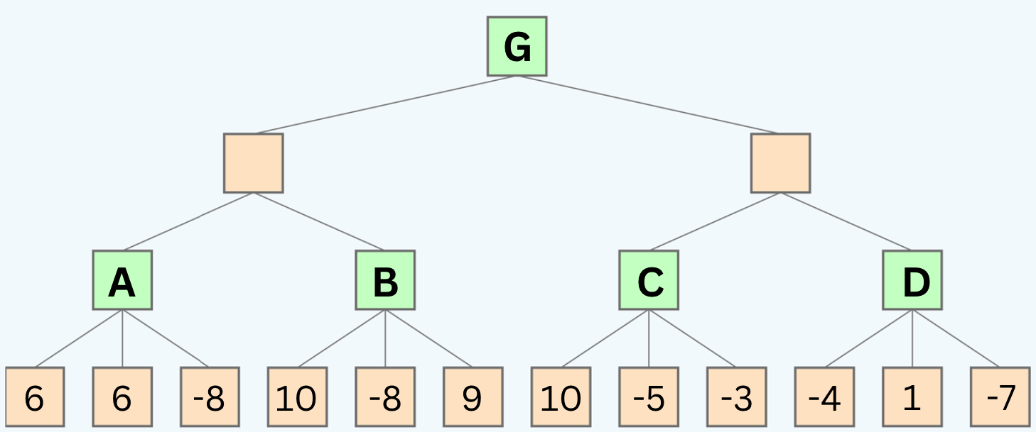
Questions:
- 1: If we use alpha-beta pruning, what are the values of the nodes labeled A, B, C, and G?
- 2: If we use alpha-beta pruning, which nodes will be pruned?
Note: that the tree is 4 levels deep, not 3. So from top to bottom, the player alternates between MAX and MIN 4 times.
Take your time to trace the algorithm on the above tree before seeing the staff solution below. Remember, this is a crucial step in your learning process. Don't rush through it.

🧩 Unfold the solution below and match it with your solution.
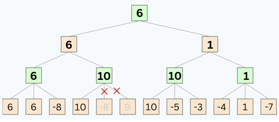
Solution
- 1: After running the whole algorithm, the values of the nodes are:
A = 6 , B = 10, C = 10, D = 1, G = 6
- 2: The nodes that will be pruned are: -8 , 9
2) Depth-Limiting
Another optimization technique is depth-limiting. Depth-limiting is a way of limiting the depth of the search tree. In other words, we can stop searching after a certain number of moves. This is a very simple technique, but it can be very effective.
In fact, it is used in many games, including chess. In chess, the depth limit is usually set to 3 or 4 moves. This is because the number of possible moves in chess is so large that it is not practical to search the entire tree. Applying depth-limiting requires an evaluation function to estimate the utility of a state when the depth limit is reached.
Heuristic Evaluation Functions
A heuristic evaluation function is a function that estimates the utility of a state without doing a complete search (without looking at all of the possible moves). Suppose that, due to limited computational resources, we can only reach a depth of 3 in our search tree. In this case, we need an evaluation function to estimate the utility of the states at that depth level.
Examples of Heuristics:
In chess, a simple heuristic is to count the total value of pieces on the board for each player. Each piece is assigned a value (e.g., pawn = 1, knight = 3, rook = 5, etc.), and the player with a higher total value is generally considered to be in a better position. This heuristic helps to evaluate the board's utility without exploring every possible future move.
In pathfinding problems, such as finding the shortest path in a maze, a common heuristic is the straight-line distance from the current position to the goal. This heuristic helps to prioritize which paths to explore first, even without searching the entire maze.
In games like Connect Four, a heuristic could be the number of three-in-a-row combinations each player has, as these are one step away from a winning four-in-a-row. This helps to estimate the utility of a board state by highlighting positions close to winning, without needing to explore every game continuation.
We can use any of these heuristics to estimate the utility of a state at a given depth without further exploring the tree. The better the heuristic, the better the estimate.
Watch this video to learn more about these optimization techniques:
If you need more explanation, watch these 2 videos:
More Optimization Techniques
Besides the above optimization techniques, there are many other techniques that can be used to improve the performance of our algorithms. Here are some of them:
Dynamic Programming: Breaks the problem down into simpler sub-problems and stores the results of these sub-problems to avoid redundant calculations. This is particularly useful for problems exhibiting overlapping subproblems and optimal substructure.
Iterative Deepening: Combines the space efficiency of depth-first search with the completeness of breadth-first search. It incrementally increases the depth limit until the goal is found.
Simulated Annealing: An optimization technique that tries to avoid getting stuck in local optima by allowing less optimal moves in the early stages of the search.
Beam Search: A heuristic search algorithm that is a combination of BFS and DFS but limits the number of children expanded at each level, keeping only a predetermined number of best nodes at each level.
Branch and Bound: Used in optimization problems, this technique systematically enumerates candidate solutions by splitting them into smaller subsets (branching) and using bounds to eliminate suboptimal solutions.
Bidirectional Search: This method runs two simultaneous searches—one forward from the initial state and the other backward from the goal—hoping that the two searches meet in the middle. This can dramatically reduce the search space.
Parallelization: This technique involves running multiple searches in parallel. This can be done by running multiple searches on different processors or by running multiple searches on the same processor using multithreading.
And many more...
Summary
- Optimization is a crucial part of AI. Without it, our algorithms may be too slow to be practical.
- Alpha-beta pruning is a way of finding the optimal minimax solution while avoiding searching subtrees of moves which won't be selected.
- Depth-limiting is a way of limiting the depth of the search tree. In other words, we can stop searching after a certain number of moves. This is a very simple technique, but it can be very effective.
- A heuristic evaluation function is a function that estimates the utility of a state without doing a complete search ( without looking at all of the possible moves). It works well with depth-limiting.
- Beside the above optimization techniques, there are many other techniques that can be used to improve the performance of our algorithms including: Dynamic Programming, Iterative Deepening, Simulated Annealing, Beam Search, Branch and Bound, Bidirectional Search, Parallelization, and many more...
Practice Quiz
Q1. What is the main purpose of alpha-beta pruning in the minimax algorithm?
- A) To increase the number of nodes in the search tree.
- B) To find the optimal minimax solution while avoiding unnecessary subtree searches.
- C) To evaluate heuristic functions.
- D) To implement depth-first search.
Q2. In the context of chess, why is depth-limiting used as an optimization technique?
- A) Because chess requires a complete search of the game tree.
- B) To limit the depth of the search tree due to the large number of possible moves in chess.
- C) To enhance the efficiency of the minimax algorithm.
- D) To calculate the exact number of moves ahead.
Q3. Which of the following is a better heuristic evaluation function in chess?
- A) Counting the total number of moves made by a player.
- B) Calculating the straight-line distance to the king.
- C) Counting the total value of pieces on the board for each player.
- D) The number of possible checkmates in two moves.
Q4. Which optimization technique combines the space efficiency of DFS with the completeness of BFS?
- A) Dynamic Programming
- B) Iterative Deepening
- C) Simulated Annealing
- D) Beam Search
Q5. What is a unique feature of bidirectional search compared to other search techniques?
- A) It involves breaking the problem down into simpler sub-problems.
- B) It uses a heuristic to estimate the utility of a state.
- C) It runs two simultaneous searches, one forward from the initial state and the other backward from the goal.
- D) It limits the depth of the search tree to a specific number of moves.
Please try the quiz first before jumping into the solution below.

Answer Key
- Q1. B) To find the optimal minimax solution while avoiding unnecessary subtree searches.
- Q2. B) To limit the depth of the search tree due to the large number of possible moves in chess.
- Q3. C) Counting the total value of pieces on the board for each player.
- Q4. B) Iterative Deepening
- Q5. C) It runs two simultaneous searches, one forward from the initial state and the other backward from the goal.
Game Theory
Game theory, a fascinating branch of mathematics with widespread applications in various disciplines, offers a systematic framework for analyzing strategic interactions among rational decision-makers. Originating from economics, game theory has evolved to become a crucial tool in fields such as political science, biology, sociology, and artificial intelligence. At its core, game theory investigates how individuals, referred to as players, make decisions when their outcomes depend not only on their own choices but also on the actions of others. It explores scenarios where conflicting interests or cooperation shape the dynamics, emphasizing the interplay of strategies and the resulting outcomes.
Notable concepts within game theory include Nash equilibrium, where no player has an incentive to change their strategy unilaterally, and the distinction between zero-sum and non-zero-sum games, where the sum of gains and losses is either constant or variable. The pervasive influence of game theory underscores its significance in unraveling the complexities of decision-making, offering valuable insights into human behavior and strategic reasoning across a spectrum of real-world scenarios.
Optional: Watch this video on game theory:
Game Playing in AI
The evolution of game-playing artificial intelligence (AI) has marked significant milestones in the realm of computational achievement.
In 1950, the world witnessed the emergence of the first computer player for checkers.
The year 1994 saw a historic moment when the computer program Chinook became the first-ever computer champion, ending the remarkable 40-year reign of human champion Marion Tinsley. Utilizing a complete 8-piece endgame, Chinook's victory marked a pivotal moment in the intersection of artificial intelligence and board games.
The landmark event continued in 2007 when checkers, as a game, was declared solved by computational methods.
Chess, a game long regarded as the pinnacle of intellectual prowess, witnessed a groundbreaking event in 1997 when Deep Blue defeated human champion Gary Kasparov in a six-game match. Deep Blue's computational capabilities were awe-inspiring, examining 200 million positions per second and employing sophisticated evaluation methods, some undisclosed, to extend search lines up to 40 ply.
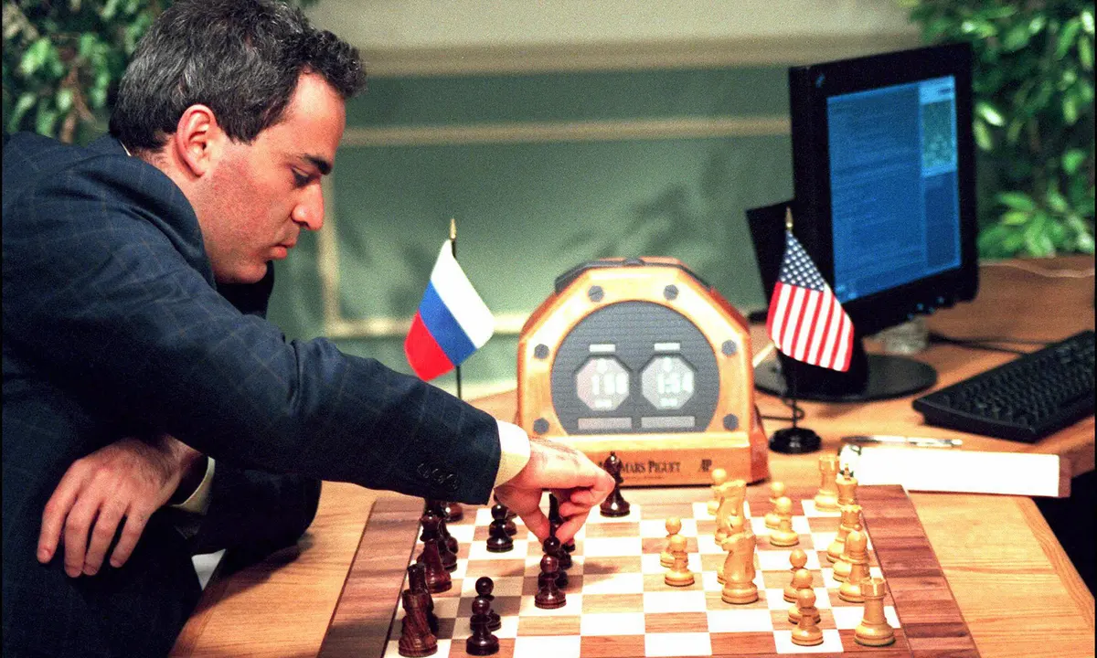 Deep Blue computer beats world chess champion – archive, 1996
Fast forward to 2016, and the game of Go experienced a revolution with AlphaGo defeating a human opponent. AlphaGo's success was attributed to its utilization of Monte Carlo Tree Search and a learned evaluation function.
These triumphs in game-playing AI underscore the instrumental role of games in tracking the progress of artificial intelligence, offering tangible benchmarks for advancements in computational abilities and strategic decision-making.
Different Types of Games
Deterministic games are those in which the outcome is fully determined by the moves of the players. Games like chess, checkers, and Go are deterministic.
Stochastic games are those in which chance or randomness is involved in the outcome of the game. Games like backgammon, snakes and ladders, and Monopoly are stochastic.
Zero sum games are those in which the sum of the payoffs of all players is zero. In other words, the gain of one player is equal to the loss of the other player. Chess, checkers, and tic-tac-toe are zero sum games.
Perfect information games are those in which the players have complete information about the state of the game at any point in time. Chess, checkers, and tic-tac-toe are perfect information games. Poker, on the other hand, is not a perfect information game because the players do not know the cards held by the other players.
Practice Problems
You may choose one of the following problems to practice your skills, or you can tackle both if you prefer. The first problem is a video tutorial on how to implement a Connect 4 AI using the minimax algorithm. The second problem is ...
Problem 1 : Connect 4 AI
Here is a complete video tutorial on how to implement a Connect 4 AI using the minimax algorithm. The tutorial is in Python.
Although this is a lengthy video, it is worthwhile. You will gain a lot of insights!
How to get the most out of this tutorial:
-
Download the starter code and get familiar with it.
-
Try to implement the minimax algorithm on your own. Push yourself harder than you think necessary. It's okay if you don't succeed at first. Just give it your best effort.
-
Watch the video without coding along. Try to understand the code and the algorithm while looking at the starter code you downloaded.
-
Try one more time to implement the minimax algorithm on your own. You should be able to do a good part of it now, if not all of it.
-
Watch the video again and code along. Pause the video from time to time to try to implement the code on your own.

Problem 2 : Checkers AI
In this problem, you will implement a Checkers AI using the minimax algorithm.
How to get the most out of this tutorial:
-
Download the [starter code]from the video description section and get familiar with it.
-
Try to implement the algorithm on your own. Push yourself harder than you think necessary. It's okay if you don't succeed at first. Just give it your best effort.
-
Watch the video without coding along. Try to understand the code and the algorithm while looking at the starter code you downloaded.
-
Try one more time to implement the minimax algorithm on your own. You should be able to do a good part of it now, if not all of it.
-
Watch the video again and code along. Pause the video from time to time to try to implement the code on your own.
Week 2 Quiz
Before attempting the quiz, read the following carefully.
- This is a timed quiz. You will have only one attempt.
- You will have 40 minutes to complete multiple-choice questions.
- You should first study the lesson materials thoroughly. More specifically, you should learn about search problems, search problem formulation, tracing and running search algorithms, and heuristic functions.
➡️ Access the quiz on OnlineExamMaker here.
Coding Assignment 2: Tic-Tac-Toe with Minimax-Alpha-Beta Pruning
In this assignment we will be implementing the alpha-beta pruning to our minimax implementation on tic-tac-toe. This is to enhance the minimax algorithm we implemented in this week's lesson.
➡️ Access the assignment and all details here.
Extra Resources:
Constraint Satisfaction Problems

🛍️ Imagine you're given the task of designing the layout for a brand-new store. Your goal is to arrange everything—from shelves to checkout counters—in a way that maximizes customer flow and boosts sales. But, there's a catch: you have to work within the limited space of the store. How do you decide where to place each item so that customers can move freely, find what they need easily, and ensure the store can operate efficiently? This is not just a design challenge; it's a classic example of a Constraint Satisfaction Problem (CSP).
🏟️ Now, let us shift gears to sports. Think about organizing a sports league or a tournament. You need to schedule multiple games, ensuring that each team plays at different times and, possibly, at different venues. You must consider the availability of each team, the availability of the venues, and even the travel constraints for the teams. Creating a schedule that avoids any overlaps or conflicts is yet another practical application of CSPs.
🧑🏾🏫 Finally, let us look at a scenario you’re all familiar with: class timetabling in schools or universities. The challenge is to schedule all classes so that no two classes that require the same room or teacher are happening at the same time. Also, students should attend all their classes without any time conflicts. This is a complex problem involving multiple constraints that need to be satisfied simultaneously.

🧩 In each of these scenarios, we're faced with a set of problems that may seem daunting at first. But, this is where the beauty of Constraint Satisfaction Problems comes into play. CSPs are not just academic exercises; they are practical, real-world challenges that we encounter in various fields like retail, sports, and education. In this lesson, we will delve into the methods and strategies used to solve CSPs.
🚀 Let's get started!
CSPs VS Search
What we have learned so far
🔎 In the past two weeks, we discussed a class of problems that can be formulated as a set of states (configurations) and transitions between them. We called these problems search problems. Our goal was to find a sequence of transitions (via actions) that leads from the initial state to a goal state. We have seen how to model these problems and how to solve them using different search algorithms.

We've also learned about situations where we have two agents competing against each other. While discussing this type of search problems, we learned about game theory and adversarial search. We have seen how to model them as games, and how to solve them.
We've also learned about optimization techniques that are very helpful in solving search problems like heuristics, pruning, depth-limiting, and more.
This week, we will discuss a different class of problem called constraint satisfaction problems (CSPs).
🗺️ Suppose that we have a map of 7 adjacent countries, and we want to color each country with one of 3 colors. We want to make sure that no two adjacent countries have the same color. How can we do that? Is this a search problem?

Well, we can perfectly think of this problem as a search problem. We can define the states as the different ways of coloring the countries. We can define the actions as coloring a country with a color. We can define the initial state as the state where no country is colored and so on. But, if you think a bit deeply, this is not a good way to model this problem. Why? Because, we would end up with a huge search space where the problem is actually simpler. Here are a few things to consider:
- We don’t need a sequence of actions to solve this problem; we can assign colors to countries in any order as the sequence does not affect the outcome.
- We don’t need to search for a goal state; instead, we need to find a viable solution.
- The color of a country doesn't depend on the color of other countries. However, there is a constraint that restricts the colors that a country can take based on the colors of its neighbors.
So, we can model this problem in a different way that's more suitable and more efficient.
What is a CSP?
A constraint satisfaction problem (CSP) is a problem where we have a set of variables (like the 7 countries to be colored), each with a domain of possible values (like Red, Green, and Blue), and a set of constraints that restrict the values that these variables can take (i.e. no two adjacent countries can have the same color). You can think of CSPs as a specialized search problems.
Our goal is to find an assignment of values to variables that satisfies all the constraints.
Summary:
-
Constraint satisfaction problems (CSPs) are a specialized class of search problems that can be modeled as a set of variables, each with a domain of possible values, and a set of constraints that restrict the values that these variables can take. We will learn more powerful techniques to solve these problems that perform better than the search algorithms we learned before.
-
Our goal is to find an assignment of values to variables that satisfies all the constraints.
Modeling CSPs
Modeling the problem, or giving it a mathematical definition, is the first step in solving it. As we did with search problems, we started by formulating the definition of the problem by stating the states, actions, and transitions, then we used algorithms to solve this general model we built.
Similarly, in CSPs, we will start by formulating the definition of the problem by stating the variables, domains, and constraints; then we will use algorithms to solve this general model we built.
Map Coloring Problem Modeling
Let's start with a simple example of a CSP: the map coloring problem. The goal is to color a map in such a way that no two adjacent regions have the same color. Available colors are red, green, and blue. Below is a map of Australia that we will use to illustrate the problem.
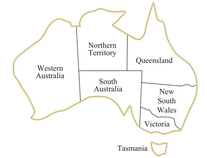
To model this problem as a CSP, we need to define the variables, domains, and constraints.
-
Variables: Each region on the map is a variable. In this case, we have seven variables:
WA, NT, Q, NSW, V, SA, and T. -
Domains: The domain of each variable is the set of colors that can be assigned to it. In this case, the domain is
D = {red, green, blue}. -
Constraints: The constraints are the rules that must be satisfied. In this case, the constraint is that no two adjacent regions can have the same color. One possible way to model this is to just write all rules of the pairs of adjacent regions like this:
- WA ≠ NT (WA and NT must not have the same color)
- WA ≠ SA (WA and SA must not have the same color)
- NT ≠ SA (NT and SA must not have the same color)
- NT ≠ Q (NT and Q must not have the same color)
- SA ≠ Q (SA and Q must not have the same color)
- SA ≠ NSW (SA and NSW must not have the same color)
- SA ≠ V (SA and V must not have the same color)
- NSW ≠ Q (NSW and Q must not have the same color)
- NSW ≠ V (NSW and V must not have the same color) This will be translated to a piece of code that checks if the constraints are satisfied.
-
Solutions: Solutions to this problem are assignments that satisfy all the constraints. For example, one possible solution is
{WA=red, NT=green, Q=red, NSW=green, V=red, SA=blue, T=green}.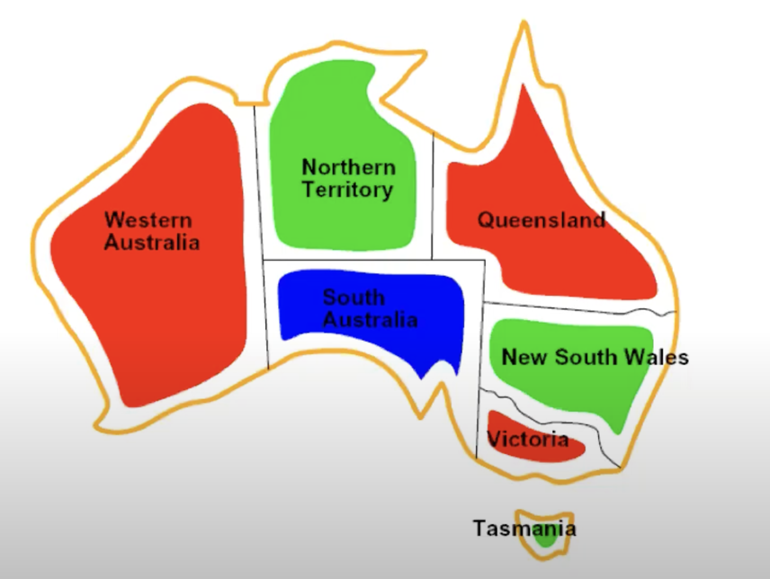
N-Queens Problem Modeling
The N-Queens problem is a classic example of a CSP. The goal is to place N queens on an N x N chessboard in such a way that no two queens are attacking each other. In other words, no two queens should be in the same row, column, or diagonal. Below is an example of a solution for N = 4.
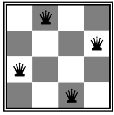
Can you think of a way to model this problem as a CSP? Remember, we need to define the variables, domains, and constraints.
Give it a try before checking the solution below.

Click here to see the solution
Here's one way to model the N-Queens problem as a CSP:-
Variables: We can consider the cell indices on the board to be our variables. In this case, we have 16 variables:
x1, x2, x3, ..., x16. -
Domains: The domain of each variable will be either 0 or 1. 0 means that there is no queen in this cell, and 1 means that there is a queen in this cell. So the domain is
{0, 1}. -
Constraints: The constraints here are that no two queens can be in the same row, column, or diagonal. We can model this constraint like that:
- Sum Constraint: The sum of each row must be equal to 1.
- Sum Constraint: The sum of each column must be equal to 1.
- Diagonal Constraint: No two queens should threaten each other diagonally.
In code, this would typically be implemented as a function that verifies these constraints on the board.
The same problem can be modeled in a different way. For example, we can consider the queens as variables and the cells as domains.
Modeling Sudoku
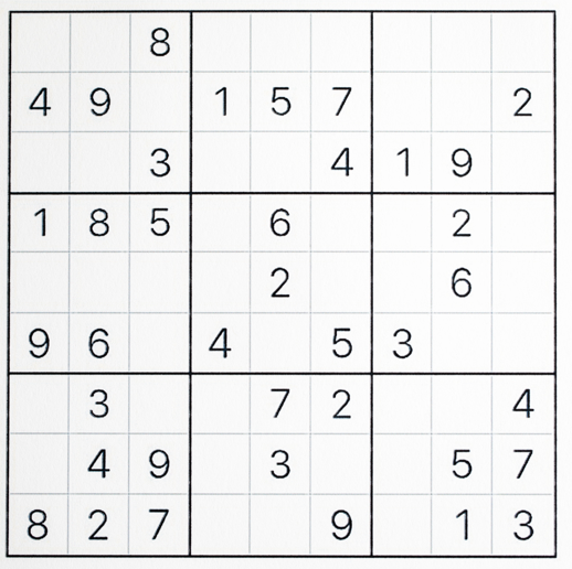
Can you think of a way to model the Sudoku problem as a CSP? Remember, we need to define the variables, domains, and constraints. Give yourself 15 minutes to think about it before checking the solution below.

Solution
Here is one possible way to model this problem:- Variables: Each cell on the Sudoku board is a variable. In this case, we have 81 variables:
x1, x2, x3, ..., x81. - Domains: The domain of each variable is the set of numbers that can be assigned to it. In this case, the domain is
{1, 2, 3, 4, 5, 6, 7, 8, 9}. - Constraints: The constraints here is that no two cells in the same row, column, or 3x3 subgrid can have the same value. We can model this constraint like that:
- Row Constraint: Each row must contain exactly one of each digit (9-way alldiff for each row).
- Column Constraint: Each column must contain exactly one of each digit (9-way alldiff for each column).
- Subgrid Constraint: Each 3x3 subgrid must contain exactly one of each digit (9-way alldiff for each subgrid) In code, it could be as simple as a function that checks the board for theses constraints.
Constraint Graph
Another helpful way to model CSPs is to use a constraint graph. A constraint graph is a graph where each node represents a variable and each edge represents a constraint. For example, here is the constraint graph for the map coloring problem we discussed earlier.
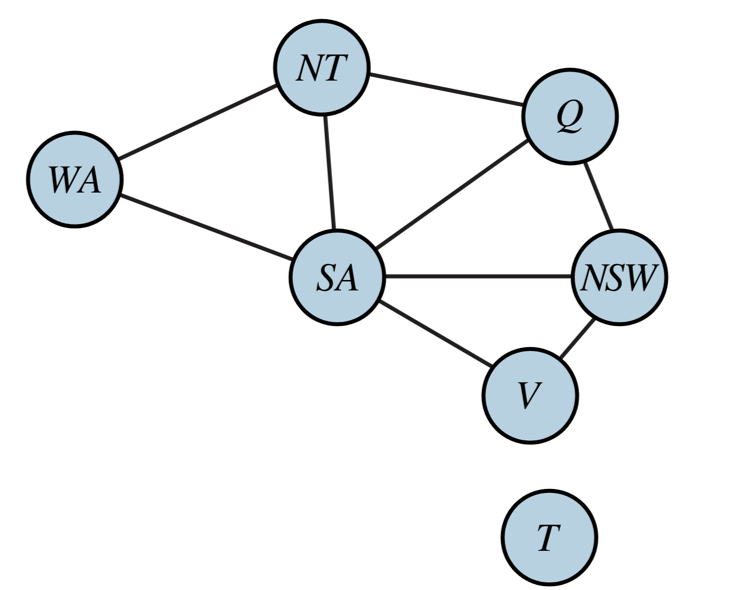
This graph shows the variables as nodes and the constraints as edges. For example, the edge between WA and NT represents a constraint. It does not say what the constraint is, but it tells us there is a constraint between these two variables. The same goes for the other edges.
The graph modeling tool can help us optimize our solution. For example, if we look at the graph above, we can see that the variable T is disconnected from the rest of the graph. This means we can work on this part of the graph separately from the rest of the graph. More on that later.
In case we have constraints that involve more than two variables, we can use a different notation. For example, if we have a constraint that says that the sum of the values of three variables must be equal to 10, we can represent it like this:
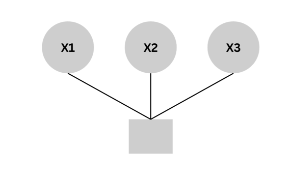
This graph tells us that there is a constraint between the three variables X1, X2, and X3. This might be helpful in other scenarios as well.
Summary
-
Constraint satisfaction problems (CSPs) are a specialized class of search problems that can be modeled as a set of variables, each with a domain of possible values, and a set of constraints that restrict the values that these variables can take. We will learn more powerful techniques to solve these problems that perform better than the search algorithms we learned before.
-
We can model CSPs by identifying the variables, domains, and constraints of the problem.
-
Finding a solution to a CSP is finding an assignment of values to variables that satisfies all the constraints.
Solving CSPs
Now that we know how to model a CSP, let's look at how to solve it.
Backtracking Search
Backtracking Search is a general algorithm that can be used to solve any CSP. The idea is to assign values to variables one at a time, and backtrack when we reach a dead end. The mechanism of the backtracking search algorithm is similar to depth-first search (DFS) algorithm. The difference is that backtracking search will backtrack when it reaches a dead end (and we have a way to check that), while DFS will continue to search until it reaches the end.
Let's start by solving the map coloring problem using backtracking search.
Remember, the goal is to color a map in such a way that no two adjacent regions have the same color. Available colors are red, green, and blue. Below is a map of Australia that we will use to illustrate the problem.
Watch how we solve the problem in the video below:
Notes on the video:
-
The first step is to select an unassigned variable. We started with
WA. We did not consider every possible configuration from that initial empty assignment. We just pickedWAand started exploring the possible values for it.
-
From this point, we will explore the possible values for
WAone at a time (red, green, and blue). At this point, we did not check every possible value from the initial assignment.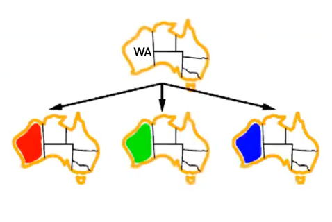
-
From the
WA = redbranch, we will only explore the values for NT that are consistent with the constraints. Some assignments, such as WA = red and NT = red, are not consistent with the constraints, so we will not explore them.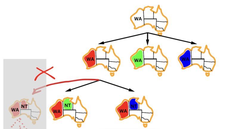
-
Link to the demo tool used in the video: CSP Demo
Let's Code It!

Here is the pseudocode for backtracking search:
![]()
Here is the code in Python:
🎉 Congratulations!🎉
You've just learned a way to solve CSP. You can see that the algorithm has found a solution to the map coloring problem.
Solving CSPs Part 2
In this lesson, we will try to improve the performance of our backtracking algorithm used in the previous lesson.
Decision Points
Remember when we tried to improve our search algorithms in previous weeks? We looked at the points where there is a decision to be made and tried to make better decisions at that point.
Can you tell what the decision points are in the search algorithms we studied?
Can you tell what the decision points are in the backtracking algorithm we studied in the previous lesson?
Similarly, we can improve our backtracking algorithm by making better decisions at the points where there is a decision to be made. In the case of CSPs, the decision points are the points where we choose a value for a variable.
Forward Checking
The first improvement, called forward checking, involves removing values inconsistent with the constraints from the domains of unassigned variables and checking if any domains become empty as a result. If any of the domains is empty, then we know that we cannot find a solution, so we backtrack.
This is the part of the pseudocode where we will add the forward checking:
add {var = value} to assignment
We will add the forward checking after selecting an unassigned variable. Here is the pseudocode:
add {var = value} to assignment

for each unassigned var in ORDER-DOMAIN-VALUES(var, assignment, csp) do
   if value is not consistent with assignment given then
        remove value from DOMAIN[var]
Here is a demo of this idea:
Notes on the video:
- The demo tool used in the video: CSP Demo
Here is the code in Python:
The output of the code is:
{'WA': 'red', 'NT': 'green', 'SA': 'blue', 'Q': 'red', 'NSW': 'green', 'V': 'red', 'T': 'green'}
To measure the performance of the algorithm, we can count the number of times we check the consistency of a value with the assignment. Add a counter variable to the code and increment it every time we check the consistency of a value with the assignment.
Here is the code with the counter:
consistency_check_counter = 0


def consistent(var, value, assignment, csp):
  global consistency_check_counter
  consistency_check_counter += 1

  for other in assignment:
    if other != var and not csp['constraints'](var, other, value,
                                               assignment[other]):
      return False
  return True
If you print the counter after running the code, you will get 7 in the forward checking case and 11 in the backtracking case. So forward checking is better than backtracking in this case.
Constraint Propagation
The second improvement is quite harder to understand. So, if you have been following along, you need to take before moving on.
Arc
An arc is a pair of variables that are connected by a constraint. For example, in the map coloring problem, the pair (WA, NT) is an arc because there is a constraint between them.
Examples arcs in the map coloring problem:
- (WA, NT)
- (NT, WA)
- (NT, SA)
- (SA, NT)
- ...
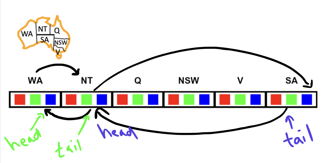
As you can see, arcs have directions. So (WA, NT) is not the same as (NT, WA).
Arc Consistency
An arc X->Y is consistent if for every value in the domain of X, there exists a corresponding value in the domain of Y that does not violate the constraint between X and Y.
In the below image, is the arc (NT, WA) consistent?
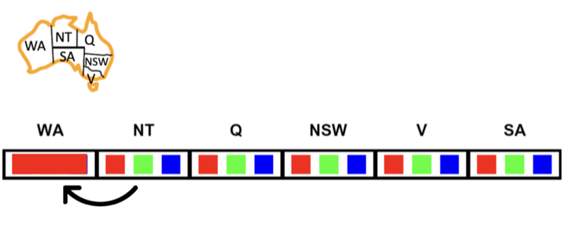
The answer is No. Why? Because WA has a value of red and the value red in the domain of NT violates the constraint between NT and WA. So the arc (NT, WA) is not consistent.
How to make it consistent? We need to remove the values from the domain of X that violate the constraint between X and Y. So, in this case, we need to remove red from the domain of NT.
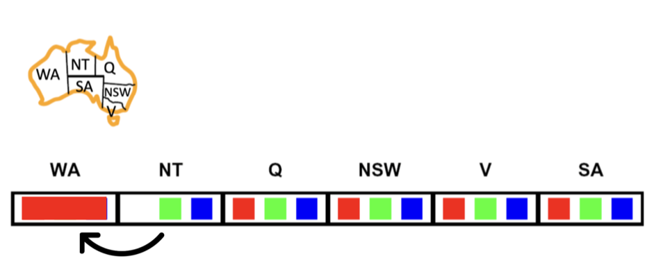
Now, it is consistent.
What about this arc?
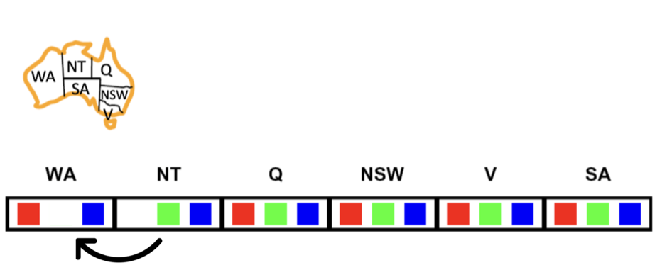
Click here to see the answer
The answer is Yes.Both the blue and green values in the domain of NT have a value in the domain of WA that does not violate the constraint between NT and WA. So the arc (NT, WA) is consistent. The available value for the NT's blue value is green from the WA domain. The available values for the NT's green value is blue and red.
Can we make all the arcs consistent? Yes, we can. We can make all the arcs consistent by removing the values from the domains of the variables that violate the constraints between them. This process is called arc consistency and this is the second improvement we will look at.
How to make all the arcs consistent?
Watch this video to see how to make all the arcs consistent:
Here is pseudocode for the algorithm for making all the arcs consistent. It is called AC-3:
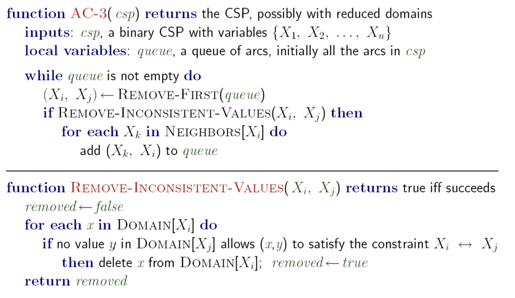
Ordering and Problem Structure
There are two additional strategies to enhance the performance of CSP solving algorithms. The first one is to choose the variables in a different order. The second one is to examine the structure of the problem and use that information to improve the performance of the algorithm. Let's discuss these two ideas briefly.
Ordering
While solving the map coloring problem, we chose the variables in the order they appear in the list of variables. Will choosing a different order affect the performance of the algorithm? It turns out that it does. Instead of choosing the variables in the order they appear in the list of variables, we can choose the variables in the order of the number of constraints on the variable. This is called the least constraining value (LCV) heuristic. Another heuristic is to choose the variable with the fewest remaining values in its domain. This is called the minimum remaining values (MRV) heuristic.
Problem Structure
The structure of the problem can provide us with information that can help us improve the performance of the algorithm. For example, if the problem is a tree-structured CSP, then we can solve it in polynomial time with less runtime and space complexity.
This is all what we need you to know about Ordering and Problem Structure. If you want to learn more about these two ideas, you can watch this video.
Summary
The effectiveness of algorithms used to solve CSPs can be significantly improved by optimizing decision-making at critical points within the search process.
- We can improve the performance of the algorithm by removing the values that are inconsistent with the constraints from the domains of the unassigned variables and then check if any of the domains is empty. If any of the domains is empty, then we know that we cannot find a solution, so we backtrack. This is called forward checking.
- Another idea is to make all the arcs consistent. This is called arc consistency. We can make all the arcs consistent by removing the values from the domains of the variables that violate the constraints between them.
- The third idea is to choose the variables in a different order. Choosing the variables in the order of the number of constraints or the fewest remaining values in its domain can improve the performance of the algorithm.
- The fourth idea is to examine the structure of the problem and use that information to improve the performance of the algorithm.
Iterative Improvement
Now, let's discuss a very interesting idea that can be used to solve not only constraint satisfaction problems but many other problems as well. It is not related to the backtracking algorithm or the improvements we discussed in the previous lesson.
Iterative Improvement
The idea is very simple, yet very powerful. It is based on the observation that we can solve the problem by starting with a random solution and then trying to improve it by making small changes to it. Let's see how it works.
Consider the map coloring problem: we begin with a random color assignment for each region. For example:
{'WA': 'blue', 'NT': 'green', 'SA': 'green', 'Q': 'red', 'NSW': 'green', 'V': 'red', 'T': 'red'} .
This initial setup reveals constraint violations among NT, SA, and NSW, due to adjacent regions sharing the same color.
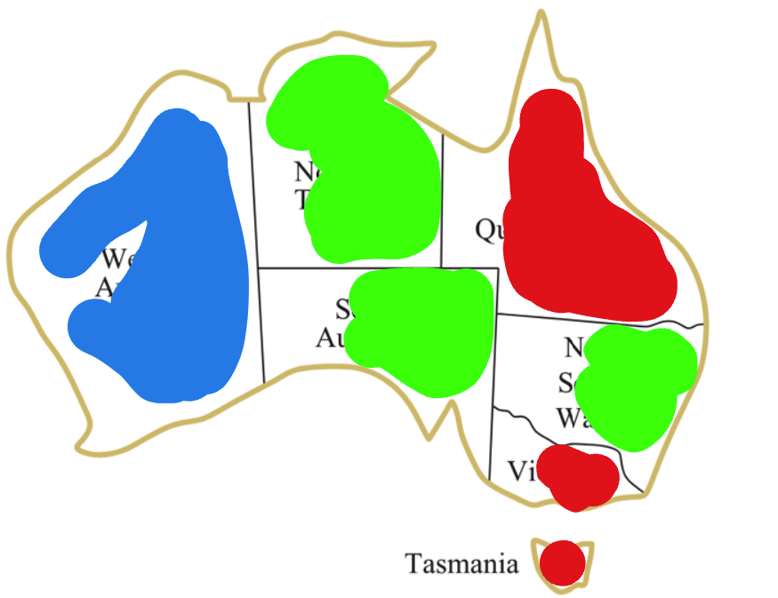
Now, we can try to improve this solution by changing the color of one of these regions. We can apply different strategies to choose which region to change. For example, we can choose the region with the highest number of constraint violations. In this case, it is SA.
Let's change the color of SA to red, resulting in a new assignment:
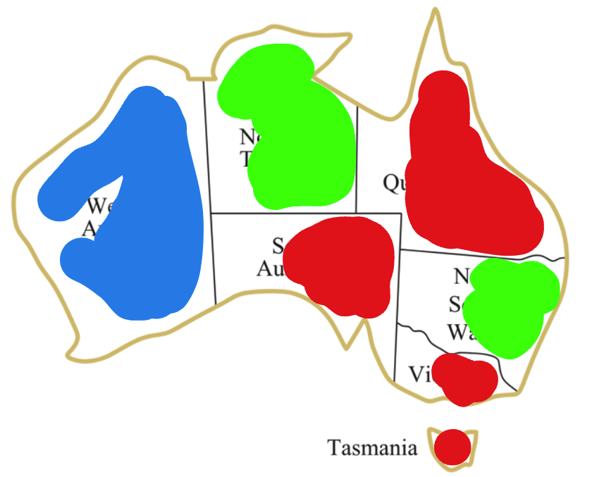
Now, we can see there are constraint violations between Q, SA, and V. The region with the highest number of constraint violations is SA. Let's change the color of SA to be blue. This will result in a new assignment:
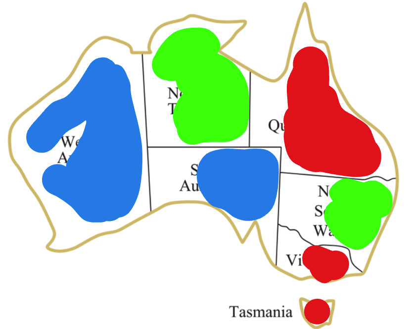
Now, we can see there is a constraint violation between WA and SA. The number of constraint violations is 1 in both. We've just changed the SA, let's try to change the color of WA this time to be red. This will result in a new assignment:
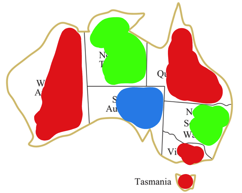
Now we have no more constraint violations. So this is a solution to the problem.
Watch this video on Iterative Improvement
Start at time: 1:07:13
Notes on Iterative Improvement Video
- The demo link: CSP Demo
- Iterative Improvement starts by assigning random values to the variables. Then it tries to improve the solution by making small changes to it.
- While the solution is not found, it keeps making small changes to the solution until it finds a solution or it reaches a maximum number of iterations.
- The variables to fix can be chosen randomly, or based on some heuristic.
- Iterative Improvement is effective in practice.
Practice - Exam Scheduling
Kibo is planning to make exams this semester for year 2 students. Kibo team wants to make the exam schedule such that no student has to take more than 1 exam on the same day. Below is a sample list of students and the courses they are taking. There are 3 days available for exams (Tuesday, Wednesday, and Thursday).
- Aisha is taking OOP , AI, and CN
- Dodze is taking AI and DB, and FED
- Joshy is taking CN, FED, and SE
- Sakira is FED, SE, and HCI
Can you help Kibo team to make the exam schedule for the students?
It is very important to try to solve the problem on your own before looking at the solution below.
Step 1: Formulate the problem as a CSP
Solution
Variables: {OOP, AI, CN, DB, FED, SE, HCI}
Domains: {Tuesday, Wednesday, Thursday}. Each variable can take one of these values.
Constraints:
- OOP != AI, OOP != CN, AI != CN,
- AI != DB, AI != FED, DB != FED,
- CN != FED, CN != SE, FED != SE
- FED != SE, FED != HCI, SE != HCI
Here is the constraint graph for the problem. Each node represents a variable (course) and each edge represents a no equality constraint (no two courses can be scheduled on the same day).
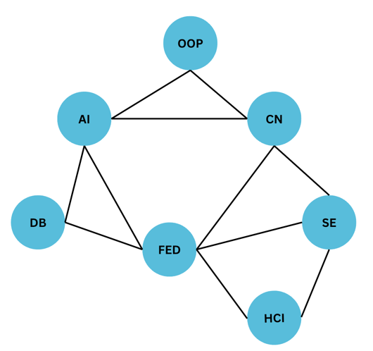
Step 2: Solve the problem using backtracking search
Step 2.1: Represent the variables in code
Solution
    courses = ["OOP", "AI", "CN", "DB", "SE", "FED", "HCI"]
    days = ["Tuesday", "Wednesday", "Thursday"]
    CONSTRAINTS = [("OOP", "AI"), ("OOP", "CN"), ("AI", "CN"), ("AI", "DB"),
               ("AI", "FED"), ("CN", "FED"), ("CN", "SE"), ("DB", "FED"),
               ("FED", "SE"), ("FED", "HCI"), ("SE", "HCI")]
Step 2.2: Represent the constraints check in code
Hint: This is a function that takes the assignment and returns True if the assignment is consistent with the constraints and False otherwise.
Solution
def is_consistent(assignment):
  """Checks to see if an assignment is consistent."""
  for (x, y) in CONSTRAINTS:

    # Only consider arcs where both are assigned
    if x not in assignment or y not in assignment:
      continue

    # If both have same value, then not consistent
    if assignment[x] == assignment[y]:
      return False

  # If nothing inconsistent, then assignment is consistent
  return True
Step 2.3: Implement the backtrack search algorithm
Hint: This is a recursive function that takes the list of variables, the current assignment, and the schedule so far. It returns the schedule if it's complete and valid, and returns False otherwise.
Solution
def backtrack_search(courses, days, assignment):
  if len(assignment) == len(courses):
    return assignment  # All courses are assigned

  current_course = next(course for course in courses
                        if course not in assignment)
  for day in days:
    if is_consistent(assignment):
      assignment[current_course] = day
      result = backtrack_search(courses, days, assignment)
      if result is not None:
        return result
      del assignment[current_course]  # Backtrack if the assignment is not consistent
  return None
Putting it all together
Solution
CONSTRAINTS = [("OOP", "AI"), ("OOP", "CN"), ("AI", "CN"), ("AI", "DB"),
               ("AI", "FED"), ("CN", "FED"), ("CN", "SE"), ("DB", "FED"),
               ("FED", "SE"), ("FED", "HCI"), ("SE", "HCI")]


def is_consistent(assignment):
  """Checks to see if an assignment is consistent."""
  for (x, y) in CONSTRAINTS:

    # Only consider arcs where both are assigned
    if x not in assignment or y not in assignment:
      continue

    # If both have same value, then not consistent
    if assignment[x] == assignment[y]:
      return False

  # If nothing inconsistent, then assignment is consistent
  return True


def backtrack_search(courses, days, assignment):
  if len(assignment) == len(courses):
    return assignment  # All courses are assigned

  current_course = next(course for course in courses
                        if course not in assignment)
  for day in days:
    if is_consistent(assignment):
      assignment[current_course] = day
      result = backtrack_search(courses, days, assignment)
      if result is not None:
        return result
      del assignment[
          current_course]  # Backtrack if the assignment is not consistent
  return None


def solve_schedule():
  courses = ["OOP", "AI", "CN", "DB", "FED", "SE", "HCI"]
  days = ["Tuesday", "Wednesday", "Thursday"]
  assignment = {}

  result = backtrack_search(courses, days, assignment)
  return result


if __name__ == "__main__":
  solution = solve_schedule()

  if solution:
    for course, day in solution.items():
      print(f"{course}: {day}")
  else:
    print("No solution found.")
Week 3 Quiz
Before attempting the quiz, read the following carefully.
- This is a timed quiz. You will have one attempt.
- You will have 25 minutes to complete multiple-choice questions.
- You should first study the lesson materials thoroughly. More specifically, you should learn about modeling CSPs, the algorithms to solve them, and the optimization techniques used to improve the solution performance.
➡️ Access the quiz here
Policy
The policy π is a function that maps a state to an action. Being in state s, what action should the agent take? After figuring out the reward function, the agent can solve an optimization problem to find the optimal policy. The optimal policy is the policy that maximizes the reward.
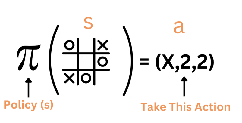
So the policy is our solution to the problem. The policy is a function, or a look-up table, that maps a state to an action.
Timing
Because actions are taken in a sequence, we represent the timing of the actions by adding a time index t to the state s and action a. For example, the state s at time t is st. The action a at time t is at.
So the states are s0, s1, s2, ... and the actions are a0, a1, a2, ....
The goal of reinforcement learning is to design a policy π that, given a state st, tell us what actions to take to maximize the reward.
Putting it all together.
Watch the video below (~10 minutes) to reiterate and better understand the concepts we discussed above.
The concepts of the Value Function and the Discount Factor explained in the video will be discussed in more detail in the next section.
Summary
-
Reinforcement learning is a type of machine learning that enables an agent to learn in an interactive environment by trial and error using feedback from its own actions and experiences.
-
Reinforcement learning framework consists of the following key elements:
- Agent
- Environment
- States
- Actions
- Reward Function
- Policy
- Value Function
-
The goal of the reinforcement learning agent is to maximize the expected total reward it receives by learning a policy
π(s)that maps states to actions.
Markov Decision Processes
Now that we have learned about the Reinforcement Learning (RL) framework, let's discuss how we can formulate a problem as an RL problem using the Markov Decision Process (MDP) formalism.
Markov Decision Processes (MDPs) provide a mathematical framework for modeling decision making in situations where outcomes are partly random and partly under the control of a decision maker.
The word "Markov" in MDP refers to the fact that the future can be determined only from the present state (i.e., the future is independent of the past).
A Markov decision process formalism consists of the following elements:
-
A set of states s ∈ S: The different states the agent/world can be in. For example, in autonomous helicopter flight, the states might be the set of all possible positions and orientations of the helicopter. In a simple grid world, the states might be the set of all possible positions (cells) of the robot.
-
A set of actions (A): The set of actions the agent can take. For example, the set of all possible directions in which you can push the helicopter’s control sticks or move the robot in the grid world (
up,down,left,right). -
A reward function R: The reward function is a function of the state. It returns the reward value of being in a state
s. The notation for the reward function isR(s),R(s,a), or R(s,a,s').s'is the state you reach after taking an action a while being in a states. -
A transition probability model Pa(s,s'): is the probability of reaching the next state
s'(pronounced s-prime) if we take actionawhile being in states. Sometimes, the transition probability model is notated asP(s'|s,a)orT(s,a, s'). You can think of it as the model of the world.In the helicopter flight example, if the helicopter is in state
sand we push the control sticks in a certain direction, the helicopter will move in that direction with some probability as the helicopter might be affected by the wind.If a robot is moving in a simple grid world, being in a certain position/cell let's say cell
1,2and you want to move it to position2,2. The world grid model might tell us that each action you take has an0.8probability of being executed successfully. So, when we direct the robot to move up, the robot might move up with a probability of0.8, move right with a probability of0.1, or move left with a probability of0.1.
Simple Grid World Example
To explain the MDP formalism, let's consider a simple MDP. The agent is in a grid world and can move up, down, left, or right. The agent receives a reward of -0.2 for each step and a reward of 10 for reaching the goal. The agent receives a reward of -5 for reaching the cliff. The agent can't move outside the grid world and can't move into the wall.
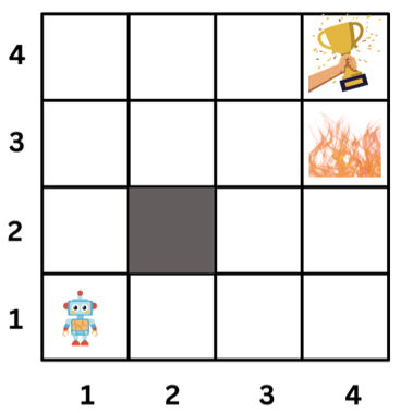
What are the elements of the MDP for this grid world?
-
States are the 15 cells in the grid world. State (2,2) is blocked.
-
Actions are the four directions the agent can move (up, down, left, right).
-
Transition Probability: In this example, we will model our world such that the agent will move in the direction it chooses with probability
0.8. The agent will move in a random direction with probability0.2. For example, if the agent chooses to move up, it will move up with probability0.8and move left or right with probability0.1each. So, the transition probability model is as follows:P(s' = (1, 2) | s = (1, 1), a = up) = 0.8: Being at state (1, 1) and taking action up, the probability of ending up at state (1, 2) is 0.8.P(s' = (1, 1) | s = (1, 1), a = up) = 0.1: Being at state (1, 1) and taking action up, the probability of ending up at state (1, 1) is 0.1.P(s' = (0, 1) | s = (1, 1), a = up) = 0.1: Being at state (1, 1) and taking action up, the probability of ending up at state (0, 1) is 0.1.
-
Reward Function: To incentivize the robot to reach the goal cell, we will put a
+10reward there. Also, to discourage the robot from falling off the cliff, we will put a-5reward there. The robot will receive a-0.2reward for each step.R(s) =-0.2for all states except the goal and the cliff.
The -0.2
is like charging the robot for each step it takes.
The robot should try to minimize the number of steps
it takes to reach the goal.
Policy
The goal of the Markov Decision Process is to find a good policy π for the decision maker. A policy is a function that maps states to actions (π: S → A). The policy tells the agent what action to take in each state. The goal is to find the policy that maximizes the expected total reward.
Optimal Policy: The optimal policy is the policy that maximizes the expected total reward. The optimal policy is denoted by π*. Below is an example of an optimal policy.
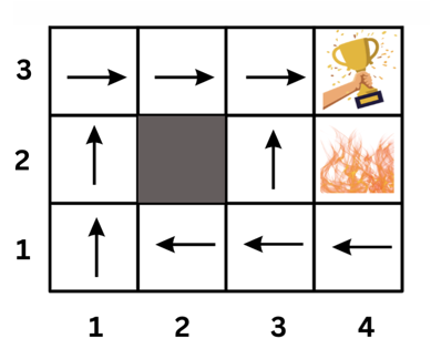
What this policy says is, for example, if the agent is at state (2,1), it should go left. That is π(2,1) = left
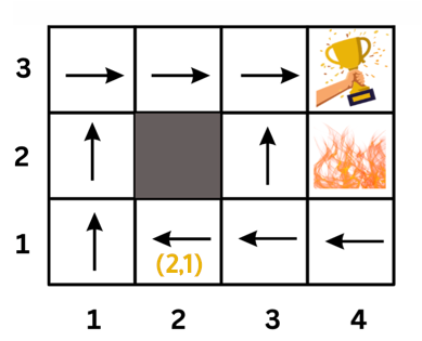
An interesting position to examine in the previous policy is position (3,1). You might think that the optimal policy is to go up because that path is shorter. However, if the agent goes up, there is a 0.1 probability that it will end up at the cliff (moving right after moving up). So the safer path is to go left and then up.
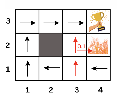
Note that this policy is heavily dependant on the transition probabilities we assumed for our world. If the transition probabilities change, the optimal policy could change too.
Solving the MDP problem is finding the optimal policy.
Markov Decision Process (MDP) Videos:
Here are some (optional) videos that explain the same concepts above. If you feel you need more explanation, you can watch them.
Discount Factor (γ)
Another important concept in MDPs is discounting. It addresses the fact that future rewards are worth less than immediate rewards. It is reasonable for agents to prefer immediate rewards over future rewards and to look forward to maximizing their total reward.
In MDPs, we use a discount factor γ (gamma) to discount future rewards. It is a value between 0 and 1 and it decays after each step.
Here is a formula that shows how the discount factor is used to calculate the expected total reward:
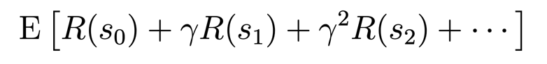
E is the expected total reward the agent will receive if it starts at state s0.
Note that we don't discount the immediate reward R(s0). We discount the future rewards by multiplying them by multiples of γ. the discount factor value decays after each step by multiplying the future rewards by multiples of γ: γ, γ^2, γ^3, γ^4, and so on.
Example:
- If we have a sequence of rewards:
r0 = 1,r1 = 2, andr2 = 3, what is the expected total utility of this sequence of rewards if:- No discounting is used?
- If
γ = 0.5?
Click here to see the answer
-
If no discounting is used, the expected total utility is
1 + 2 + 3 = 6. -
If
γ = 0.5, the expected total utility is1 + 2*0.5 + 3*0.5^2 = 2.75.
Discounting Quiz:
In the image below, we have 5 states: a, b, c, d, and e. The reward function is R(s) = 0 for all states except a and e. R(a) = 10 and R(e) = 1. You can move right or left.
You can also exit from state a or e. The environment is deterministic (transition probability is 1). Answer the questions below.
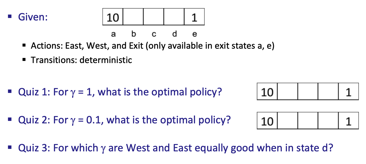
Reference: Berkeley CS188 Intro to AI
- Your answer should be in the form of a policy. For example, if you are at state
b, you should moveleft. If you are at statec, you should moverightetc. Think about the total reward you will get at each state taking into account the discount factorY.
Click here to see the answers
Q1: For Y = 1 (No Discounting):- If I'm at state
a, I willexitand get reward of 10. - If I'm at state
b, I will moveleftbecause the sum of rewards is 10 (0+10). - If I'm at state
c, I will moveleftbecause the sum of rewards is 10 (0+0+10). - If I'm at state
d, I will moveleftbecause the sum of rewards is 10 (0+0+0+10). - If I'm at state
e, and have the option to moveleftor exit, I will move left because the sum of rewards is 10. quiz-policy1.png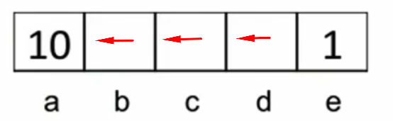
Q2: For Y = 0.1:
-
If I'm at state
a, I will exit and get reward of 10. -
If I'm at state
b, I will move left because the sum of discounted rewards is 1 (0+0.1 * 10). If I move right, the sum of discounted rewards is 0.001 (0.1^0*1). -
If I'm at state
c, I will move left because the sum of rewards is 0.1 (0+0.1*0+0.1^2 * 10). If I move right, the sum of rewards is 0.001 (0+0.1 * 0+0.1^2 * 0+0.1^3 * 10). -
If I'm at state
d, I will moverightbecause the sum of rewards is 0.1 (0+0.1). If I move left, the sum of rewards is 0.001 (0+0.1 * 0+0.1^2 * 0+0.1^3 * 10).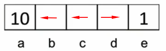
Q3: Solving the linear equation 0Y+ 0Y^2 + 10Y^3 = 1*Y, we get Y = 0.316.
Summary:
- Markov Decision Processes (MDPs) provide a mathematical framework for modeling decision making in situations where outcomes are partly random and partly under the control of a decision maker.
- The word "Markov" in MDP refers to the fact that the future can be determined only from the present state (i.e., the future is independent of the past).
- A Markov decision process formalism consists of the following elements: a set of states S, a set of actions A, a reward function R, and a transition probability model P.
- The goal of the Markov Decision Process is to find a good policy π for the decision maker. A policy is a function that maps states to actions (π: S → A). The policy tells the agent what action to take in each state. The goal is to find the policy that maximizes the expected total reward.
- The optimal policy is the policy that maximizes the expected total reward. The optimal policy is denoted by π*.
- The discount factor is a value between 0 and 1 and it decays after each step. It is used to model the fact that the future rewards are worth less than its value due to the delay in receiving them.
MDP Exercise
Blackjack
Blackjack is a card game where the goal is to beat the dealer by obtaining cards that sum closer to 21 (without going over 21) than the dealer's cards. The game starts with the dealer having one face up and one face down card, while the player has two face up cards. All cards are drawn from an infinite deck.
The card values are:
- Face cards (Jack, Queen, King) have a point value of 10.
- Aces can either count as 11, which is referred to as a 'usable ace', or as 1, depending on which value benefits the player's hand more.
- Numerical cards (2-10) have a value equal to their number.
The player has the sum of cards held. The player can request additional cards (hit) until they decide to stop (stick) or exceed 21 (bust, immediate loss).
After the player sticks, the dealer reveals their facedown card, and draws cards. If the dealer goes bust, the player wins.
If neither the player nor the dealer busts, the outcome (win, lose, draw) is decided by whose sum is closer to 21.
If you are not familiar with Blackjack, I would suggest to look at the following rules of Blackjack and try a few games online.
Questions:
1. What are the states and the actions for this MDP?
2. Give an example of a possible reward and a possible transition probability.
⚠️ Please try to solve the exercise before looking at the solution. This is important for your learning.
Click here for hints
-
In a certain point in time during the game, what states we have in terms of the score of the players. What about winning?. Look at this screenshot from a blackjack game:

-
What are are the available actions for the user to take?
Click here to see the solution
Q1 :
-
Sates:
- Each state has the player's current total hand value, the dealer's visible card value, and whether the player has a usable Ace or not.
- The state space includes all valid combinations like: (7,14,False), (5,7,True). Each tuple represents the player's current sum, the dealer's facing card value, and whether or not the player has a usable Ace.
- The possible values for the player's current sum range from 4 to 21. The minimum sum of 4 assumes scenarios where the lowest cards are drawn, like two 2s, and does not account for the flexibility of the Ace being used as 1 or 11. The dealer's facing card value can be any value from 1 to 10. The player's usable Ace can be either True or False.
- The "bust" state is an extra state that happens when the player's total exceeds 21 (for example, the user has the cards 5 and 10, then draws another card whose value is 10. This will make a total of 25 (bust)).
-
Actions: The actions available to a player in our model of Blackjack are typically "Hit" and "Stick"
Q2 :
-
The reward structure in Blackjack is:
- Winning a hand in Blackjack results in a reward equal to the bet placed. For simplicity, we can make a reward of
1for the winning state. - Losing a hand results in losing the bet. For simplicity, we can make a reward of
-1for the losing state. - A draw results in a reward of
0(no change in the player's money (the bet is returned)).
- Winning a hand in Blackjack results in a reward equal to the bet placed. For simplicity, we can make a reward of
-
The transition function in Blackjack defines the probability of moving to state s' after taking an action a. For example, the probability of reaching the state (17, 8, False) from the state (10, 8, False), when a hit action is taken, is modeled like this:
P(s' = (17, 8, False) | s = (10, 8, False), a = 'hit') = 0.077. This probability assumes a reshuffled or effectively infinite deck where the likelihood of drawing a 7, with 8 such cards in a 104-card deck, remains constant.
Solving MDPs
Now that we have defined the MDP formalism, we can use it to solve reinforcement learning problems. The goal of the reinforcement learning agent is to maximize the expected total reward it receives by learning a policy π(s) that maps states to actions. So, given an MDP, how do we find the optimal policy? This is what we will learn in this lesson.
Policy
Recall that a policy is a function (π) that maps from the states to the actions. We say that we are executing some policy π if, whenever we are in state s, we take action a = π(s).
In our previous grid world example, an example of a policy is shown below:
π((1, 1)) = up
π((1, 2)) = up
π((1, 3)) = right
π((2, 1)) = left
π((2, 3)) = right
π((3, 1)) = left
π((3, 2)) = left
...
Thus, at any given state, the policy directs us on which action to take.
In a simple 4x4 grid world, there are 16 states and 4 actions per state. This results in 416 , which is over 4 billion possible policies.
Value Iteration Algorithm
There are different algorithms that can be used to find the optimal policy (solving MDPs). The algorithm we will use in this lesson is called value iteration.
Value iteration is a dynamic programming algorithm that computes the optimal state value function by iteratively improving the estimate of a value function V(s).
But, what is the value function V(s)? Let's find out.
Value Function V(s):
The value function V(s) tells us the expected total payoff (rewards) upon starting in a state s. These values are not known in advance. We have to learn them, as we will see later.
The optimal value function V*(s) is the maximum value function over all possible policies. If we can solve for the optimal value function V*(s), we can find the optimal policy π* which is the policy that maximizes the value function V*(s).
Here is an image that shows a sample value function output of each state:
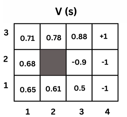
Calculating the Values of the States
The value of each state is the expected total payoff (rewards) upon starting in that state. That is the immediate reward being at this state plus the discounted future rewards of the next states.
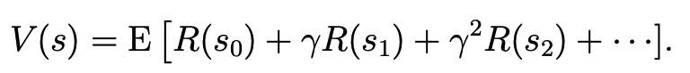
Which is equivalent to the general form using s and s' as follows:
V(s) = E [ R(s) + γ * V(s')]
That means the value function of state s is the immediate reward R(s) plus the value function value of the next state `s' taking into account the probability of reaching that state. So we can use the following formula to express that:
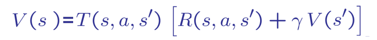
Where: T(s, a, s') is the probability of reaching state s' from state s taking action a.
In fact, we can reach different states from the same state s by taking different actions. So, we sum over all possible states s' that we can reach from state s. Then, to get the optimal value function, we take the maximum value of all possible actions.
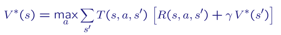
Now, you might want to read the previous section again! It's a bit confusing at first, but it will make sense as we go.
If you feel you need more explanation, you can watch this video that explains the value function and the value iteration algorithm in detail:
Stop at time 49:00
Example:
Assume that a robot in a 4x4 grid world and the transition probabilities are as follows:
- Each action has a 0.8 probability of moving in the intended direction and a 0.2 probability of moving in each of the other directions.
- The discount factor
γis 0.9 - The immediate reward
R(s)is0for all states except the cup state which has a reward of1and the fire state which has a reward of-1.
Given the above information, we can calculate the value function of each state using the Bellman equation as follows:
V(s) = R(s) + γ * Σs' Pss' * V(s')
Initially, the value function of each state is zero. Then, we take steps to update the values using the Bellman equation. So, V0(s) = 0 for all s.
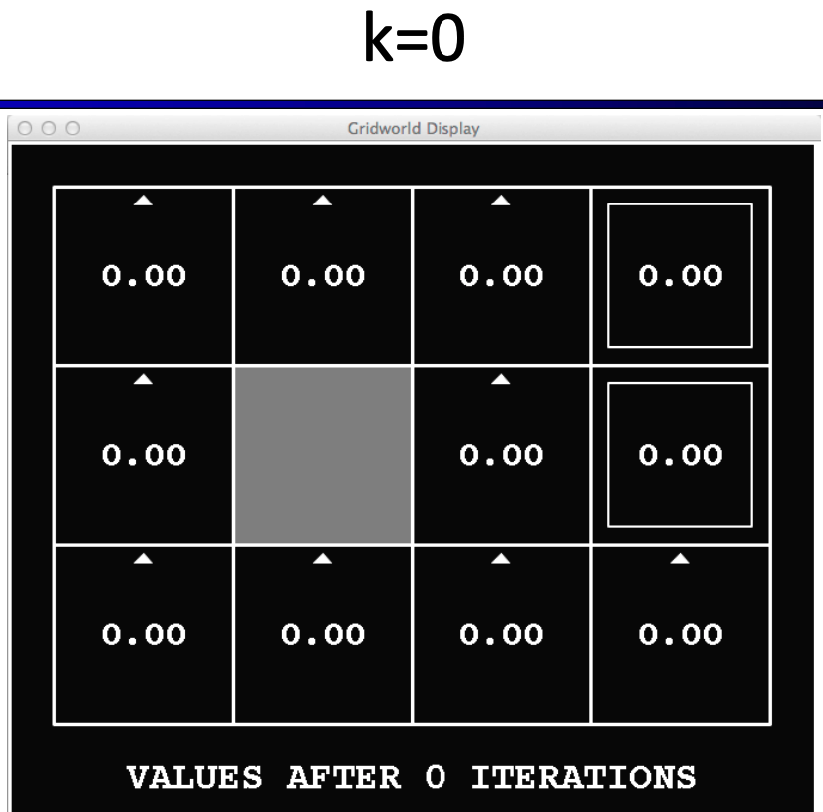
Then, starting from V1(s), we can calculate the value function of each state using the Bellman equation. For example, let's calculate the value function of state (1,1):
State (1,1):
We have 2 possible actions: up and right. If we take the up action, we have a 0.8 probability of moving to state (1,2) and 0.1 probability of moving to each of the other states.
V(s=(1,1), a="up") = 0 + 0.9 * (0.8 * V(s=(1,2)) + 0.1 * V(s=(1,1)) + 0.1 * V(s=(2,1))) = 0 because the current values of V(s=(1,2)) and V(s=(2,1)) are zero.
Same for the right action:
V(s=(1,1), a="right") = 0 + 0.9 * (0.8 * V(s=(2,1)) + 0.1 * V(s=(1,1)) + 0.1 * V(s=(1,2))) = 0 because the current values of V(s=(1,2)) and V(s=(2,1)) are zero.
In this iteration, V1, most of the other states will have a value of zero as well. Let's calculate the value function of state (3,3):
V(s=(3,3), a="terminate") = 1 + 0.9 * (0.8 * 0 + 0.1 * 0 + 0.1 * 0) = 1
After 1 iteration, the value function of each state is updated as follows:
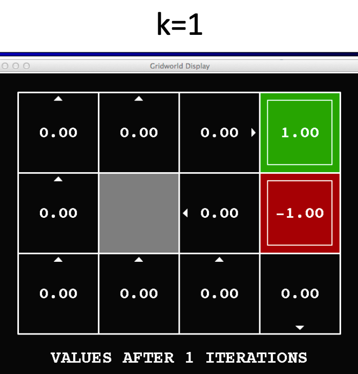
Note the arrows in the image above. For each state, we calculate the value function of each action and take the maximum value. For example, the value function of state (1,1) is the maximum value of the value function of the up action and the value function of the right action.
Doing the same calculations for the next iteration, we will end up with the following value function for V3(s):
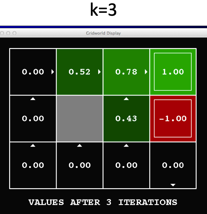
When do we stop?
We stop when the value function converges to a stable value. That is, when the value function of each state does not change much between iterations or we exceed a maximum number of iterations we set.
Value Iteration Algorithm
Now The value iteration algorithm should be clear. We start with an initial estimate of the value function V(s) and iteratively update the estimate of the value function V(s) until it converges to the optimal value function V*(s). We stop when the change in the value function is less than a threshold or we exceed a maximum number of iterations we set.
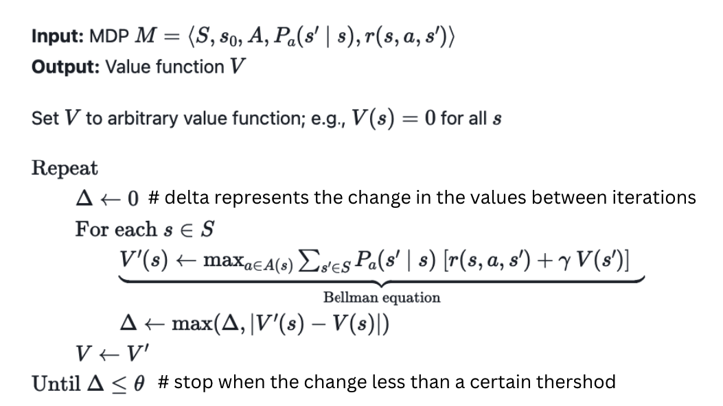
Optimal Policy
Now that we have the optimal value function V*(s), we can find the optimal policy π*. Recall that the optimal policy returns the action that maximizes the expected total reward and we know from the previous equation which action maximizes the expected total reward. So basically, we can find the action that maximizes the expected total reward and use it as the optimal policy.
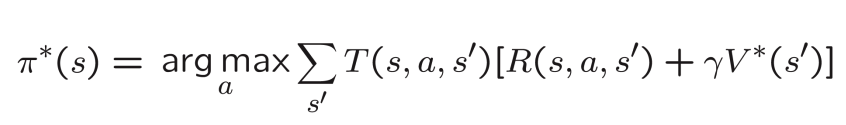
Value Iteration Mini-Blackjack
Here is a good example of running the value iteration algorithm on a simplified version of blackjack:
Note: The video has been trimmed to focus specifically on the relevant sections. It starts at 0:00 and ends at 17:35.
Value Iteration Frozen Lake Example
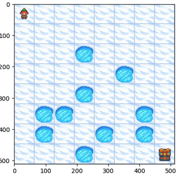
Gymnasium is an open source Python library for developing and comparing reinforcement learning algorithms. It provides a family of environments for testing reinforcement learning algorithms. Commonly used environments include the Frozen Lake environment, the CartPole environment, Blackjack environment, and the Mountain Car environment.
Each environment has an observation space and an action space. The observation space is the set of all possible states in the environment. The action space is the set of all possible actions that an agent can take in the environment.
Introduction to Gymnasium and Frozen Lake environment
Gymnasium is an open source Python library for developing and comparing reinforcement learning algorithms by providing a standard API to communicate between learning algorithms and environments. It is a fork of OpenAI's Gym library by its maintainers.
This practice lesson consists of two parts. The first part is a brief introduction to the Gymnasium library and the Frozen Lake environment. The second part is a demonstration of the value iteration algorithm on the Frozen Lake environment.
Part 1: Introduction to Gymnasium and Frozen Lake environment
Follow this colab notebook to learn about the Gymnasium library and the Frozen Lake environment. The notebook includes a brief introduction to the Gymnasium library and the Frozen Lake environment.

Quiz
After you have completed the Colab notebook, answer the following questions:
- How do you show the states and actions for the Frozen Lake environment?
- What does the variable
env.unwrapped.Prepresent in an environment? - [True/False] In the Frozen Lake environment, where the action
0means moving to the left, if the agent is in state2,2and takes action0, the agent will certainly move to state1,2.
Click here for the answers
1. You can show the states and actions for the Frozen Lake environment using the following code:print(env.observation_space)
print(env.action_space)
-
The variable
env.unwrapped.Prepresents the transition probabilities of the environment. It is a dictionary where the keys are the states, and the values are the possible actions and the next states with the corresponding probabilities. -
False. The transition probabilities are not deterministic. The agent may move to state
1,2with certain probability (0.33 in this case).
Part 2: Value Iteration on Frozen Lake environment
Follow this colab notebook to learn about the value iteration algorithm and how to apply it to the Frozen Lake environment.

Policy Iteration
Another common method for solving MDPs is policy iteration. Policy iteration operates as follows:
-
Initialize a policy arbitrarily. That means, for each state, we have to choose an action randomly.
An example of a random policy in a grid world could be:
policy = {
    (1, 1): 'up',
    (1, 2): 'up',
    (1, 3): 'Right',
    (2, 1): 'up',
    (2, 2): 'Right',
    (2, 3): 'up',
    (3, 1): 'up'
    (3, 2): 'Right'
    (3, 3): 'up'
}
This is totally arbitrary. We can choose any policy we want.
-
Policy Evaluation: Given a policy π, calculate the value function V
π for the policy π. To do this, we will do the following:
-
For each state, we calculate the value function using the following formula:
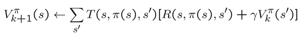
kis the number of steps we take. This means that, after taking k+1 steps, the value of the state s is the sum of the immediate reward and the discounted value of the next state. That's close to the value iteration algorithm we have seen before except that, we are not taking the action that maximizes the expected value of the next state, but we are following the policyπ. So, the immediate reward isR(s, π(s), s')which is the reward I get taking the action defined byπ(s)in statesand reaching states'. The discounted value of the next state is also calculated using the value function of the next state folowing the policyπ.The input to the value function is the policy π. The output is the value function V
π for the policy π. This is a system of linear equations that can be solved using linear algebra.
-
Policy Improvement: from the current state values we have from step1, consider all actions and choose the action that maximizes the expected values of the next states. This is the same as doing one iteration of the value iteration algorithm.
-
Policy Iteration: Repeat steps 2 and 3 until the policy converges.
Value Iteration vs Policy Iteration
For small MDPs (i.e. few hundred states), policy iteration is often very fast and converges with very few iterations. However, for MDPs with large state spaces (i.e. 10 thousands or more), solving for Vπ explicitly would involve solving a large system of linear equations, and could be difficult. In these problems, value iteration may be preferred. For this reason, in practice value iteration seems to be used more often than policy iteration.
If you feel you need more explanation, you can watch this video that explains the value function and the value iteration algorithm in detail:
You may stop at time 58:15
Solving Mini-Blackjack using Policy Iteration
Value Iteration Frozen Lake Example
To understand the application of the policy iteration algorithm in the Frozen Lake environment, please follow this Colab notebook. It provides step-by-step instructions and interactive exercises that demonstrate the algorithm's implementation.

Week 4 Quiz: Reinforcement Learning
Before attempting the quiz, read the following carefully.
- This is a timed quiz. You will have one attempt.
- You will have 40 minutes to complete multiple-choice questions.
- You should first study the lesson materials thoroughly.
➡️ Access the quiz here.
Assignment: Value Iteration on Blackjack environment
Follow this colab notebook to complete the assignment:

Submission
Submit your assignment via gradescope here
Supervised Machine Learning!

This week, we embark on an exciting journey into the world of machine learning, exploring its fundamentals and applications in various projects. Our lesson will cover a broad range of topics, including:
- The essence of machine learning
- Key types of machine learning: Supervised, Unsupervised, and Reinforcement Learning
- Regression and Classification techniques
- And more
In the previous weeks, we discussed various approaches to achieving intelligence: tweaking algorithms for improved search, modeling constraints and rules for constraint satisfaction problems (CSPs), and learning from experience and rewards in Reinforcement Learning (RL). This week, we shift our focus to deriving intelligence from data.
Intelligence by Learning from Data
Can intelligence emerge from data analysis? Absolutely. A significant portion of Machine Learning is dedicated to this very concept.
Learning from data involves developing algorithms and models capable of analyzing, interpreting, and making predictions or decisions based on data. This process requires training models on large datasets to identify patterns and relationships not immediately apparent. As models are exposed to more data, their predictive and decision-making capabilities improve.
What is Machine Learning?
The conceptual framework of Machine Learning is straightforward: we leverage data, examples, experiences, and observations to teach computers how to learn.
Arthur Samuel defined machine learning as a subfield of computer science that enables computers to learn without being explicitly programmed.
Explicitly Programmed vs. Learning from Data
-
Explicitly programmed: Writing a program for a specific task.
-
Learning from data: Providing numerous examples of inputs and outputs for the machine to learn from, enabling it to predict outputs for new inputs.
Consider the challenge of identifying a person from a photograph. Writing a program for direct comparison, such as pixel-by-pixel analysis, is impractical, due to the variability in photos. Machine learning overcomes this by using labeled photographs to teach computers to identify people in images, exemplifying AI learning.
Types of Learning:
Machine Learning encompasses three primary learning types:
-
Supervised Learning: (Classification, Regression): Learning a function that maps inputs to outputs from example input-output pairs. This includes tasks like email spam classification, tumor malignancy classification, and stock price forecasting.
-
Unsupervised Learning: (Clustering, Dimensionality Reduction): Finding patterns in unlabeled data, such as grouping customers by purchasing behavior or reducing the number of data features for efficiency.
-
Reinforcement Learning: Learning from the outcomes of actions in an environment to maximize some notion of cumulative reward.
Supervised Learning
Supervised learning is a type of machine learning predominantly used in many real-world applications, witnessing rapid advancements and innovations. It involves learning a function that maps an input to an output based on example input-output pairs, a process also known as function approximation.
This approach entails providing the machine with numerous examples of inputs and outputs (labels), enabling it to learn from these examples and predict the output for any new input. The algorithm attempts to identify patterns within the data, creating a model capable of replicating the same underlying rules with new data. Remarkable, isn't it?
Model: An algorithmic formula designed to produce an outcome with new data, based on the principles derived from the training data. Once the model is developed, it can be applied to new data and evaluated for accuracy.
Examples of supervised learning algorithms include regression analysis, decision trees, k-nearest neighbors, neural networks, and support vector machines.
Examples of supervised learning applications include:
-
Regression: Estimating a continuous value:
- Forecasting a house's price in dollars based on its features.
- Predicting a person's age based on their medical records.
- Forecasting stock prices.
-
Classification: Predicting a label (category) from a set of labels.
- Classifying an email as spam or not spam.
- Identifying a tumor as malignant or benign.
- Recognizing images of handwritten digits.
- Facilitating face recognition.
- Categorizing news articles into different categories.
Unsupervised Learning
Unsupervised learning algorithms seek patterns in unlabeled data. For instance, consider data about a company's customers where the goal is to identify patterns. The aim is to find groups of customers with similar purchasing behaviors, despite the absence of predefined labels for these groups. An unsupervised learning algorithm might determine that the data can be segmented into two distinct groups or clusters.
Examples of unsupervised learning include:
-
Clustering: Aggregating similar data points.
- Sorting customers by their purchasing habits.
- Organizing news articles by their topics.
- Grouping patients based on their medical histories.
-
Dimensionality Reduction: Decreasing the number of data features.
- Data compression: Minimizing the data size.
-
Anomaly Detection: Identifying outliers within the data.
- Detecting fraud.
- Identifying manufacturing defects.
- Diagnosing medical issues.
We will commence with supervised learning, starting with regression.
Let's dive in! 🚀
Linear Regression
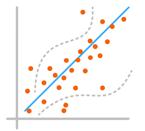
What is Regression?
In its simplest form, regression is a statistical method used to model the connection between a dependent variable and one or more independent variables. The dependent variable is the variable we aim to predict, while the independent variables are the variables used to predict the outcome.
An example of a simple regression problem is predicting the price of a house based on its size, number of rooms, and location. In this case, the price of the house is the dependent variable, while the size, number of rooms, and location are the independent variables.
The technique of regression analysis involves developing a mathematical model that describes the relationship between the dependent and independent variables.
In machine learning,the key idea behind regression is that, given that we have enough data, we can learn the relationship between the independent and dependent variables from the data. We can then use this learned relationship to predict the outcome of future events.Regression is a form of supervised learning.
Types of Regression
There are several types of regression, but the most common ones in machine learning are:
-
Linear Regression: Models the linear relationship between the dependent and independent variables. It assumes a straight-line relationship.
-
Polynomial Regression: Models the relationship between the dependent and independent variables as an nth-degree polynomial. It assumes a non-linear relationship.
-
Logistic Regression: Models the relationship between the dependent and independent variables by estimating the probability that a given input belongs to a specific category. It is used for classification problems.
We will start with One-variable Linear Regression and then move on to other types of regression in the upcoming lessons.
One-variable Linear Regression
When we have one input variable (feature), we call it one-variable linear regression. Later on, we will learn about multiple variable linear regression, in which we have more than one input variable (multiple features).
Goal
Our goal in Linear Regression is to find the best fit line (equation) that describes the relationship between the variables that can later be used to predict the outcome of future events.
Here is a sample dataset that contains the amount of money spent on advertising and the resulting sales. The goal is to predict the amount of sales based on the amount of money spent on advertising.
| Advertising | Sales |
|---|---|
| 100 | 1000 |
| 200 | 2000 |
| 300 | 3000 |
| 400 | 4000 |
| 500 | 5000 |
| 600 | 6000 |
| 700 | 7000 |
| 800 | 8000 |
Can you predict the sales when the money spent on advertising is 1170?
Data usually is not that simple. But let's illustrate the idea of regression using this simple example first and then we will move on to more complex examples.
Here is a scatter plot of the data:
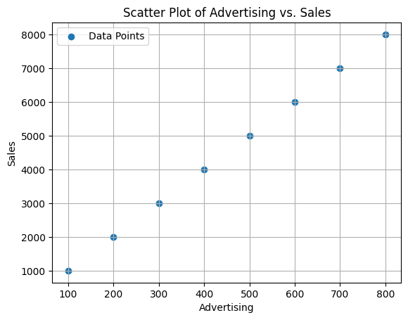
This dataset forms a perfect straight line. The equation of a straight line is Y = wX + b. The value of w is the slope of the line. The value of b is the y-intercept of the line.
Using any two points on the line, or from the data table, we can calculate the slope of the line and the y-intercept of the line. Let's use the first and the last points to calculate the slope and the y-intercept of the line.
w (slope) = (y2 - y1) / (x2 - x1) = (5000 - 1000) / (500 - 100) = 4000 / 400 = 10
We can calculate the y-intercept of the line using the slope of the line and any point on the line like this:
b = y - wx = 1000 - 10 * 100 = 1000 - 1000 = 0
So, the equation of the line is y = 10x + 0 = 10x.
Having the equation of the regression line, we can predict the outcome of any future events. For example, if you want to predict the sales when you spend 3750 on advertising, you can predict that the resulting sales will be 10 * x = 37500.
This was a very simple example but we've learned a lot.
- We learned that the equation of a straight line is
y = wx + b. - We learned the parameters of the line
wandb. - We learned how to calculate the parameters of the line.
- We learned how to use the equation of the line to predict the outcome of future events.
Example: Car Price Prediction
Here is a video that explains the basics of linear regression with a simple example. Please watch it and then we will continue our discussion.
Now, let's move on to a more complex example. Here is a part of a dataset that contains the age of a person and the insurance cost of that person.
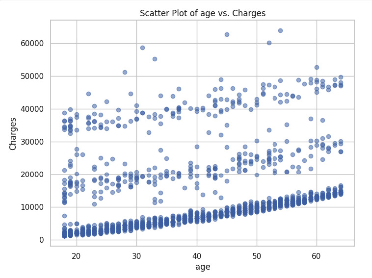
Can you predict the insurance cost of a person knowing their age? Can you draw a line on that plot that describes the relationship between the age of a person and their insurance cost 🤔?
It is not that easy, isn't it? Let's try to draw a line that describes the relationship between the age of a person and their insurance cost. Here are a few lines that I drew:
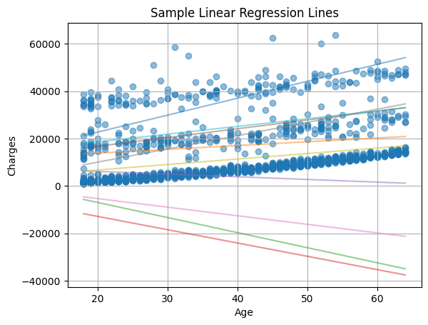
Just by looking at the graph, we can determine which lines are better than the others but, among the lines that are close to the data points, it is still not easy to determine which one is better.
Let's discuss a systematic way to determine which line is better than the others. But before we do that, let's learn how can we find these lines different lines.
Parameters
We can draw multiple candidate lines by adjusting the parameters. The line's parameters are w and b. We can experiment with different values of w and b to create different lines. Here are a few lines that I created by varying the line's parameters:
What values of w and b do we use? Initially, we'll rely on our intuition to make educated guesses about parameter values. Later on, we will utilize a technique called gradient descent to find the best parameter values for us.
Best Fit Line
How can we determine which line is the best fit? One approach to accomplish this is by calculating the distance between the data points and the line.
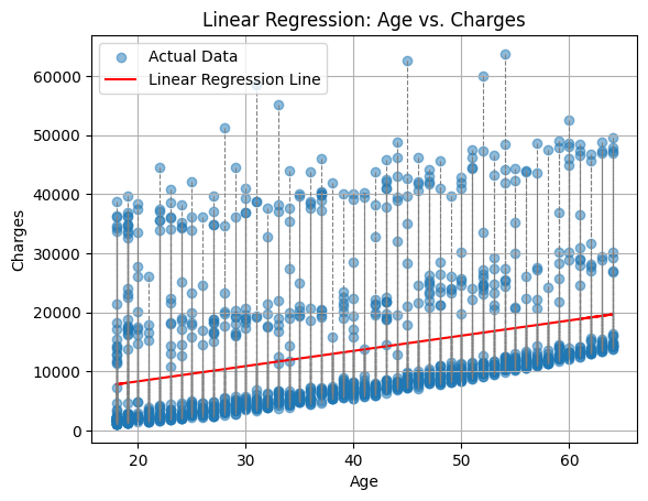
The smaller the distance between all points and the line, the better the line. This distance between a point and a line is referred to as the error.
Cost Function
Ideally, we would like the distance between the points and the line to be zero, but that is rare in real-life scenarios. Therefore, our objective is to identify the line with the smallest distances (smallest error) between the points and the line.
In a dataset showing the relationship between the age of a person and their insurance cost, here is a sample of the errors for one line:
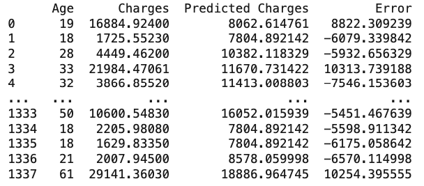
Error
As you can see, the raw data does not tell us much. We need to find a way to summarize the errors in a way that is more meaningful. The average of the errors, for example, might be a good way to summarize the errors but having negative and positive errors might cancel each other out. In practice, there is a better method called the mean of squared errors to summarize the errors. Here is the equation of the mean of squared errors:
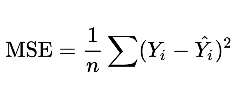
What the equation says is that we calculate the difference between the actual value and the predicted value for each point, square the difference, and then calculate the average of all the squared differences.
This is also called the cost function. The cost function is a function that maps some values of one or more variables onto a real number intuitively representing some "cost" associated with the event. This is precisely what we need to effectively utilize these error values.
If you feel you need more explanation, please watch this video.
In machine learning, we use a slightly modified version of the mean of squared errors. Here is the formula we use in machine learning:
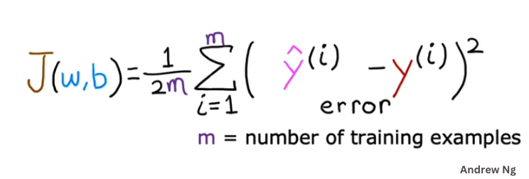
Here is the explanation of the formula:
J(w,b)is the cost function. It is a function of the parameters of the linewandb.mis the number of data points. The division by2mis to make the calculation easier.y^(i)is the predicted value of theith data pointy(i)is the actual value of theith data point∑is the summation symbol. It means we need to add all the values of the expression that follows it.
Theta Notation
In some references, the regression equation is modeled using θ0 and θ1 values instead of w and b. The equation of the line is then expressed as hθ(x) = θ0 + θ1x, where θ0 and θ1 are the y-intercept and the slope of the line, respectively. This approach stems from the assumption that our goal begins with a hypothesis, h, and we aim to find the best hypothesis that accurately describes the relationship between the variables.
The cost function, represented as J(θ0, θ1), takes the following form:
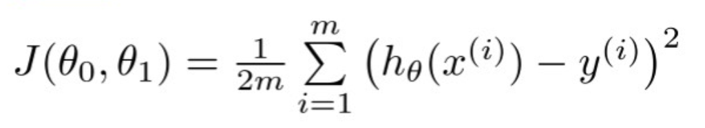
Cost Function Videos
If you feel you need more explanation of the cost function and how it is calculated, please watch the following videos:
Example:
Let's apply what we've learned so far using an example. Here is a sample dataset that contains the amount of money spent on advertising and the resulting sales. The goal is to predict the amount of sales based on the amount of money spent on advertising.
| Advertising | Sales |
|---|---|
| 100 | 1000 |
| 200 | 1400 |
| 300 | 2300 |
| 400 | 2300 |
| 500 | 3500 |
Finding the Best Fit Line
Remember that the goal of regression is to find the best fit line (equation) that describes the relationship between the variables that can later be used to predict the outcome of future events.
To do so, we need to find the parameters of the line: w and b that will find the best fit line. In other words, we need to find the values of w and b that will minimize the cost function.
Here is a manual way of finding the best fit line. We will try different values of w and b and calculate the cost function for each set of values. Then we will select the set of values that gives the smallest cost function.
Trying w =1 and b = 5
Y^ = wx + b = 1x + 5 = x + 5
| Advertising (x) | Sales (y) | w | b | y^ | y | Y^-y | (y^- y)^2 |
|---|---|---|---|---|---|---|---|
| 100 | 1000 | 1 | 5 | 105 | 1000 | -895 | 864025 |
| 200 | 1400 | 1 | 5 | 205 | 1400 | -1195 | 1425025 |
| 300 | 2300 | 1 | 5 | 305 | 2300 | -1995 | 3980025 |
| 400 | 2300 | 1 | 5 | 405 | 2300 | -1895 | 3582025 |
| 500 | 3500 | 1 | 5 | 505 | 3500 | -2995 | 8975025 |
The calculated cost function with w=1 and b=5 for our dataset is: 7,772,102.5. Seems like a very large number. Let's try another set of values for w and b.
Trying w =2 and b = 50:
| Advertising | Sales | w | b | y^ | y | Y^-y | (y^- y)^2 |
|---|---|---|---|---|---|---|---|
| 100 | 1000 | 2 | 50 | 250 | 1000 | -750 | 562500 |
| 200 | 1400 | 2 | 50 | 450 | 1400 | -950 | 902500 |
| 300 | 2300 | 2 | 50 | 650 | 2300 | -1650 | 2722500 |
| 400 | 2300 | 2 | 50 | 850 | 2300 | -1450 | 2102500 |
| 500 | 3500 | 2 | 50 | 1050 | 3500 | -2450 | 6002500 |
The calculated cost function with w=2 and b=50 for our dataset is: 1,231,000.0. Better.
Trying w =5 and b = 500:
| Advertising | Sales | w | b | y^ | y | Y^-y | (y^- y)^2 |
|---|---|---|---|---|---|---|---|
| 100 | 1000 | 5 | 500 | 1000 | 1000 | 0 | 0 |
| 200 | 1400 | 5 | 500 | 1500 | 1400 | 100 | 10000 |
| 300 | 2300 | 5 | 500 | 2000 | 2300 | -300 | 90000 |
| 400 | 2300 | 5 | 500 | 2500 | 2300 | 200 | 40000 |
| 500 | 3500 | 5 | 500 | 3000 | 3500 | -500 | 250000 |
The calculated cost function with w=5 and b=500 for our dataset is: 39,000. Much better.
Trying w =2 and b = 1000:
| Advertising | Sales | w | b | y^ | y | Y^-y | (y^- y)^2 |
|---|---|---|---|---|---|---|---|
| 100 | 1000 | 2 | 1000 | 1200 | 1000 | 200 | 40000 |
| 200 | 1400 | 2 | 1000 | 1400 | 1400 | 0 | 0 |
| 300 | 2300 | 2 | 1000 | 1600 | 2300 | -700 | 490000 |
| 400 | 2300 | 2 | 1000 | 1800 | 2300 | -500 | 250000 |
| 500 | 3500 | 2 | 1000 | 2000 | 3500 | -1500 | 2250000 |
The calculated cost function with w=2 and b=1000 for our dataset is: 319,000.0. Up again.
Trying w =2 and b = 500:
| Advertising | Sales | w | b | y^ | y | Y^-y | (y^- y)^2 |
|---|---|---|---|---|---|---|---|
| 100 | 1000 | 2 | 500 | 600 | 1000 | -400 | 160000 |
| 200 | 1400 | 2 | 500 | 800 | 1400 | -600 | 360000 |
| 300 | 2300 | 2 | 500 | 1000 | 2300 | -1300 | 1690000 |
| 400 | 2300 | 2 | 500 | 1200 | 2300 | -1100 | 1210000 |
| 500 | 3500 | 2 | 500 | 1400 | 3500 | -2100 | 4410000 |
The calculated cost function with w=2 and b=500 for our dataset is: 777,100.0. Up again.
If we decide to stop here, we can use the equation of the line y = 5x + 500 to predict the outcome of future events. For example, if you want to predict the sales when you spend 3750 on advertising, you can predict that the resulting sales will be 5 * x + 500 = 5 * 3750 + 500 = 19,750.
Results
These were 5 iterations. We tried 5 different values of w and b. The smallest cost we could get is 39,000. So, the best fit line we could find so far is the one with w=5 and b=500.
Can we do better? We can if we try more values of w and b but we will hire the computer to do that for us in the next lesson.
Welcome to Learning!
What we saw above is a core part of how machines learning algorithms works. It tries to "learn" the best fit line by trying different values of the parameters and calculating the cost function for each set of values. Then it selects the set of values that gives the smallest cost.
Solve the exercise in the next section to practice what you've learned so far.
Summary
-
Regression is a form of supervised learning employed to model the relation between one or more variables, allowing us to forecast outcomes based on this relationship.
-
The primary objective of regression is to determine the most suitable line or curve that characterizes the relationship between the variables. This regression line or curve serves as a tool to anticipate outcomes in future scenarios.
-
The equation of a straight line is
y = wx + b. The value ofwis the slope of the line. The value ofbis the y-intercept of the line. The slope of the line is the change in y divided by the change in x. The y-intercept of the line is the value of y when x is 0. -
The "cost" or "loss" function is a function that maps some values of one or more variables onto a real number intuitively representing some "cost" associated with the event. This is precisely what we need to effectively utilize these error values.
-
The common cost function used in machine learning is the mean of squared errors. Here is the formula we use:
Exercise: One-variable Linear Regression
Here is a sample dataset that contains the mid-term and final exam scores of 10 students. The goal is to predict the final exam score based on the mid-term exam score.
| Mid-term | Final |
|---|---|
| 70 | 80 |
| 80 | 90 |
| 90 | 100 |
| 60 | 70 |
| 50 | 65 |
| 40 | 50 |
| 30 | 40 |
| 20 | 30 |
| 10 | 20 |
| 0 | 10 |
Questions:
-
What is the number of features in this dataset?
-
What is the number of data points (m) in this dataset?
-
Which of these
wandbvalues will give the smallest cost function?w = 1andb = 10w = 0.5andb = 20w = 3andb = 7
-
Write a simple Python code to calculate the cost function for each set of
wandbvalues and try different values to find the smallest cost function.
Answer
-
There is only one feature (X) in this dataset which is the mid-term exam score. The final exam score is the label (Y) that we are trying to predict.
-
The number of data points (m) is 10. There are 10 students in this dataset.
-
w = 1andb = 10will give the smallest cost function. You can try that manually or use this code to calculate the cost function for each set of values:
import numpy as np

# Given dataset
mid_term_scores = np.array([70, 80, 90, 60, 50, 40, 30, 20, 10, 0])
final_scores = np.array([80, 90, 100, 70, 65, 50, 40, 30, 20, 10])

# # Calculate the mean squared error (MSE) for given values of w and b

def calculate_mse(w, b):
    predicted_final = w * mid_term_scores + b
    m = len(mid_term_scores)
    mse = (1/(2*m)) * np.sum((predicted_final - final_scores)**2)
    return predicted_final, mse

# Test cases
w_values = [1, 0.5, 3]
b_values = [10, 20, 7]

for w, b in zip(w_values, b_values):
    predicted_final, mse = calculate_mse(w, b)
    print(f"For w = {w} and b = {b}:")
    print("Predicted Final Scores:", predicted_final)
    print("Mean Squared Error (MSE):", mse)
    print()
Gradient Descent
We have learned about linear regression and how to use it to predict the value of an output variable based on the value of one input variable(feature). We have also learned about the cost function and how to use it to measure the error of the model. In this lesson, we will learn about gradient descent, a popular optimization algorithm used to minimize the cost function.
Watch the following videos in the given order:
Introduction to Gradient Descent:
Gradient Descent Implementation:
Key points from the videos:
Gradient Descent
Gradient descent is an optimization algorithm used to minimize the cost function. The cost function is a function that measures the error of the model. The cost function for linear regression is the mean of squared error.
The equation of the gradient descent algorithm is as follows:
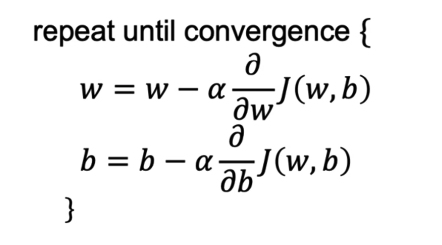
-
The idea of gradient descent is to start with a random value for the coefficients and then iteratively update the coefficients in the direction of the gradient of the cost function until we reach a local minimum.
-
The derivative term in the gradient descent equation tells us in which direction we should update the coefficients. In combination with the learning rate, the derivative term tells us how much we should update the coefficients.
-
If we are already at a local minimum, the derivative term will be zero and the coefficients will not be changed.
The Learning Rate and Number of Iterations:
- The learning rate is a hyperparameter that controls how much we update the coefficients in each iteration.
- The learning rate is usually set to a small positive number between
0and1. - If the learning rate is too small, the algorithm will take a long time to converge. If the learning rate is too large, the algorithm may overshoot the minimum and potentially never converge.
- The number of iterations is another hyperparameter that controls the number of iterations the algorithm will run. If the number of iterations is too small, the algorithm may not converge. If the number of iterations is too large, the algorithm will take a long time to converge.
Gradient Descent for Linear Regression:
Practice Quiz:
Q. Which of the following are true statements? Select all that apply.
-
To make gradient descent converge, we must slowly decrease alpha (α) over time.
-
Gradient descent is guaranteed to find the global minimum for any function J(θ0, θ1).
-
Gradient descent can converge even if α is kept fixed. (But α cannot be too large, or else it may fail to converge.)
-
For the specific choice of cost function J(θ0, θ1) used in linear regression, there are no local optima other than the global optimum.
Click here for the solution
Ans: 3, 4-
To make gradient descent converge, we must slowly decrease alpha (α) over time. (False). We don't have to decrease α over time. It can be fixed and the algorithm will still converge to the optimal value.
-
Gradient descent is guaranteed to find the global minimum for any function J(θ0, θ1). (False). Gradient descent is not guaranteed to find the global minimum for any function. It may find a local minimum instead.
-
Gradient descent can converge even if α is kept fixed. (But α cannot be too large, or else it may fail to converge.) (True). If α is too large, gradient descent may fail to converge. However, if α is small enough, gradient descent will converge even if α is not decreased over time.
-
For the specific choice of cost function J(θ0, θ1) used in linear regression, there are no local optima (other than the global optimum).( True). This is because the cost function in linear regression (mean of squared error) is convex, meaning any local minimum is also a global minimum.
Linear Regression with Multiple Variables
In our previous lessons, we learned about linear regression. More specifically, One-variable linear regression in which we had one input variable (feature) and one output variable. In this lesson, we will learn about multiple linear regression in which we have more than one input variable (multiple features). It is also known as multivariate linear regression.
Watch this video to learn about multiple linear regression:
Multiple Linear Regression
In multiple linear regression:
-
We have more than one input variable that contribute in predicting the output variable.
-
The equation of the line is a linear combination of the input variables.

Multiple Linear Regression Example
In this insurance dataset, we have the following features: age, sex, bmi, children, smoker, and region. We want to predict the charges (output variable) based on these features. Here is a sample of the data:
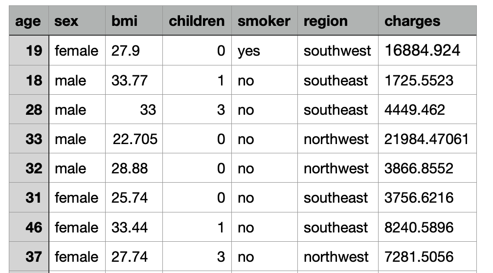
With x1, x2, ..., x6 being the age, sex, bmi, children, smoker, and region features, respectively, the equation is as follows.
fw,b(x) = w1x1 + w2x2 + .. + w6x6 + b
The model should learn the values of the coefficients w1, w2, ..., w6 that minimize the error between the predicted charges and the actual charges.
As we saw in the video, a common way to represent the features mathematically is by using vectors.
where X = [x1, x2, .. x6] and W = [w1, w2, .. w6]
Gradient Descent on Multiple Linear Regression
The gradient descent algorithm for multiple linear regression is the same as the one for one-variable linear regression. The only difference is that we have more than one coefficient to update. The gradient descent equation for multiple linear regression is as follows.
where w is a vector of the coefficients [w1, w2, ... wn] and x is a vector of the features [x1, x2, ... xn].
Watch this video to learn about gradient descent for multiple regression:
Polynomial Regression
Now that we have learned about multiple linear regression, let's see how we can use it to fit a polynomial function (a function that has a non-linear relationship between the input and output variables).
Watch this video to learn about polynomial regression:
Key points from the video:
- Polynomial regression is a form of regression in which the relationship between the variables are modeled as an nth degree polynomial.
- Feature Engineering practices are very important in regression.
Practice Regression
Follow this Colab notebook to practice regression:

Logistic Regression and Classification
In this lesson, we will learn about classification and logistic regression.
Classification
While regression is used to predict continuous values, classification is used to predict classes, such as "spam," or "not spam," or "cancer" and "no cancer," or "cat," "dog," "bird," "fish," etc.
A binary classification, a sub-type of classification, predicts a binary output {0,1}, positive and negative, or yes and no. For example, a binary classifier may predict whether an email is spam or not spam.
A multi-class classification predicts a multi-class output {0,1,2,3} or {cat, dog, bird, fish}.
Approaching Classification Problems
At its core, we are still using the regression mindset. We are still trying to find the best parameters to fit the data. The only difference is that we are trying to fit the data to a binary or multi-class output, not a continuous one.
From Regression to Classification:
Logistic Regression
Logistic regression is a classification algorithm used to assign observations to a discrete set of classes. Unlike linear regression which outputs continuous number values, logistic regression transforms its output using the logistic function to return a probability value which can then be mapped to two or more discrete classes.
The sigmoid function
As mentioned in the video, the sigmoid function is an S-shaped curve that can take any real-valued number and map it into a value between the range of 0 and 1. This is exactly what we need because we want to map the output of the regression model function to probability values between 0 and 1.
Cost Function for Logistic Regression:
Notes on the Video:
- Recall that we use gradient descent to minimize the cost function and find the best parameters for the model.
- The shape of the cost function we used for linear regression (Mean Squared Error) is convex, which means that it has only one minimum. This makes it easy to find the global minimum.
- We can't use the same cost function (MSE) for logistic regression because the resulting cost function would be non-convex. This would make it difficult to find the global minimum.
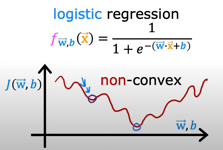
- The cost (loss) function of logistic regression is defined as:
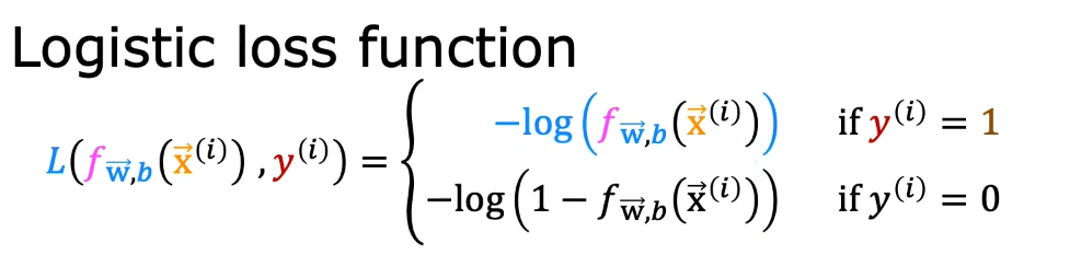
Let's now use gradient descent to minimize the cost function of logistic regression.
Gradient Descent for Logistic Regression:
Notes on the Video:
- Using the loss function of logistic regression, instead of the MSE of linear regression, we can use gradient descent to minimize the cost function and find the best parameters for the model.
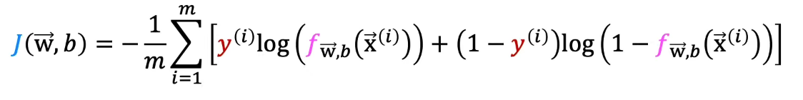
Practice Classification
Follow this Colab notebook to practice classification using logistic regression:

Model Improvement
Overfitting
In machine learning, overfitting and underfitting are two key challenges that need to be addressed to build a good model.
Watch this video to understand the concept of overfitting and underfitting.
Addressing Overfitting
Naive Bayes Classifier
In our previous lessons, we learned about the classification problem and how to solve it using the logistic regression algorithm. In this lesson, we will highlight another classification algorithm that is widely used in machine learning: the Naive Bayes classifier.
The Naive Bayes classifier is a simple probabilistic classifier based on applying Bayes' theorem with strong (naive) independence assumptions. It is a fast, accurate, and reliable algorithm that is widely used for text classification, spam filtering, and recommendation systems.
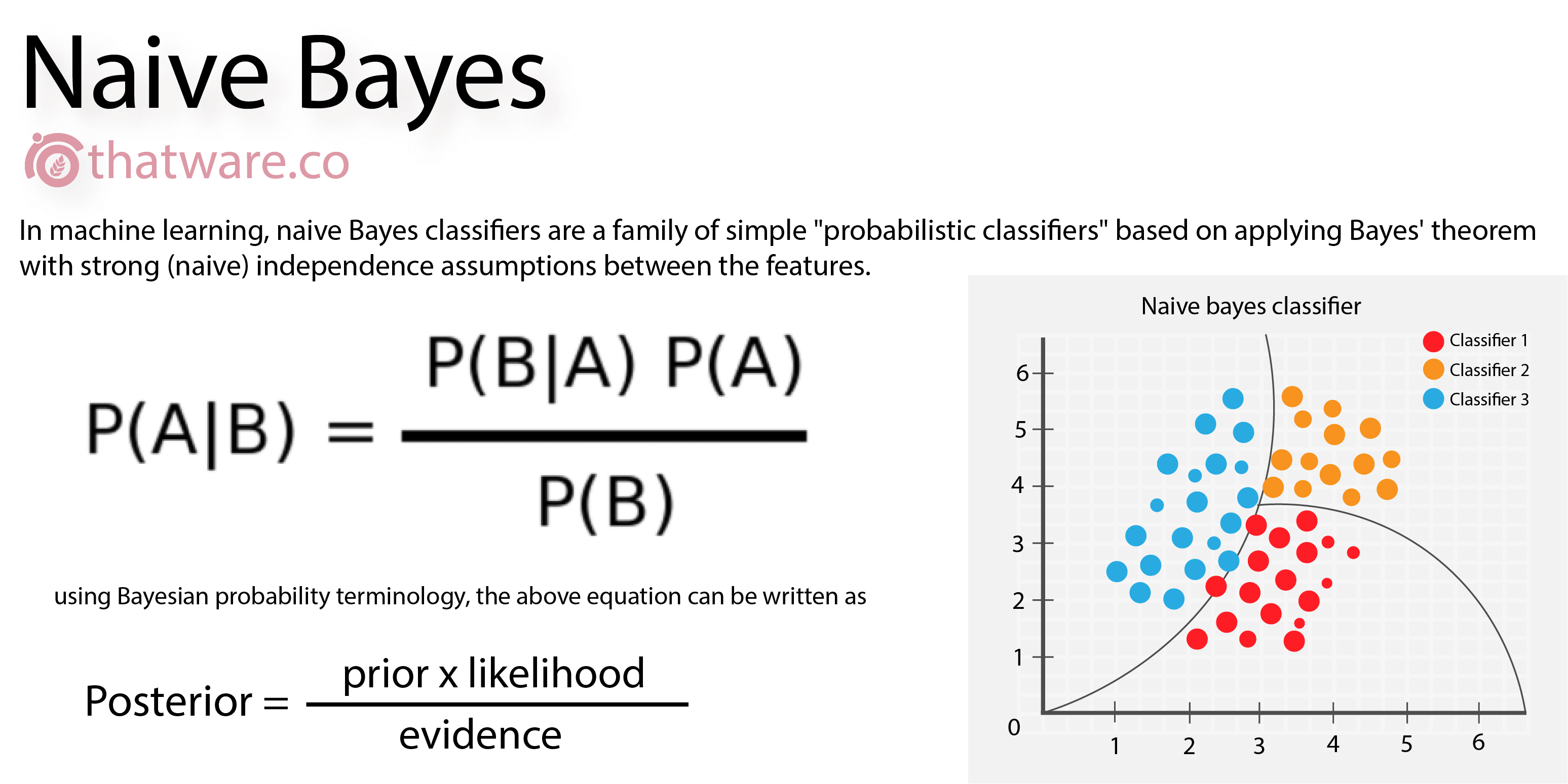
How Naive Bayes Works
Watch the following video to learn how the Naive Bayes classifier works:
Notes on the Video
-
Bayes' Theorem: It is a fundamental theorem in probability theory that describes the probability of an event, based on prior knowledge of conditions that might be related to the event. It is named after Thomas Bayes.
-
Naive Bayes Classifier: It is a simple probabilistic classifier based on applying Bayes' theorem with strong (naive) independence assumptions. It is widely used for text classification, spam filtering, and recommendation systems.
Classification Algorithms
In the last lesson, we learned about the classification problem and how to solve it using the logistic regression algorithm. In this lesson, we will highlight other classification algorithms that are widely used in machine learning.
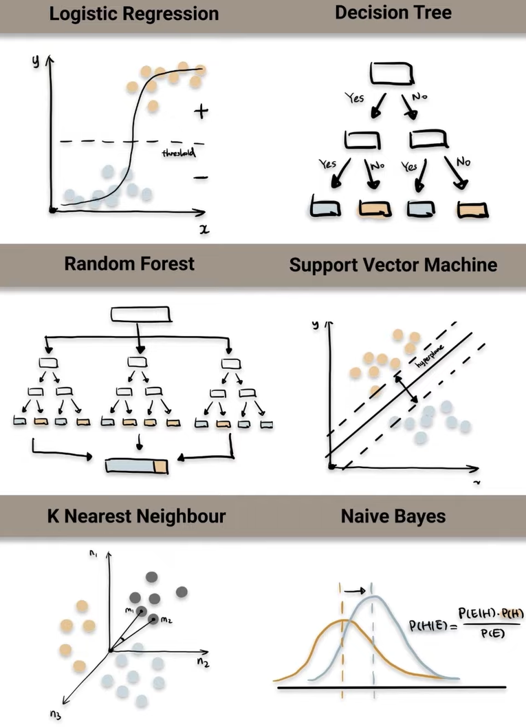
Watch this (trimmed) video to learn more about 6 common classification algorithms:
Week 5 Quiz : Machine Learning
Before attempting the quiz, read the following carefully.
- This is a timed quiz. You will have one attempt.
- You will have 20 minutes to complete multiple-choice questions.
➡️ Access the quiz here
Assignment: Naive Bayes Classifier
Your task for this assignment is to implement a Naive Bayes classifier to identify potential customers who have a higher probability of purchasing a loan.
Instructions
** A complete guide has been provided in the Colab notebook below to help you complete the assignment.**
- Use this bank_loan dataset to train and test your model.
- Create a Colab notebook and write your code in it.
- Without using any high-level libraries like
sklearnortensorflow, implement the Naive Bayes classifier to predict the potential customers who have a higher probability of accepting the personal loan offer. - The dataset contains 12 featurs and 1 target variable ("Personal Loan").
- age : Customer's age in completed years
- experience : years of professional experience
- income : Annual income of the customer
- zip_code : Home Address ZIP code.
- family : Family size of the customer
- ccavg : Avg. spending on credit cards per month
- education : Education Level (Undergrad, Graduate, Advanced/Professional)
- mortgage : Value of house mortgage if any.
- personal_loan : Did this customer accept the personal loan offered in the last campaign?
- securities_account : Does the customer have a securities account with the bank?
- cd_account : Does the customer have a certificate of deposit (CD) account with the bank?
- online : Does the customer use internet banking facilities?
- Implement basic data exploration techniques to understand the dataset.
Guide
A complete guide, including a video, has been provided in the Colab notebook below to help you complete the assignment.

Submission
- Submit your notebook link via Gradescope here
Neural Networks and Computer Vision
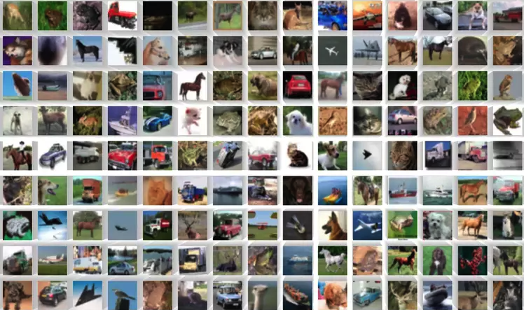
CIFAR-10 Dataset
Welcome to the fascinating world of Neural Networks! This week, we embark on an exciting journey to explore the fundamentals of neural networks and their applications across a variety of projects.
By the end of this week, you will have the opportunity to construct an image classifier using a Convolutional Neural Network (CNN). Additionally, you'll learn how to effectively train and evaluate your model using TensorFlow and Keras, two powerful tools in the field of deep learning.
Your assignment for this week will be to build a CNN model that recognizes faces
Let's dive in! 🚀
Neural Networks
Neural networks, or more specifically, artificial neural networks (ANNs), represent a computational approach inspired by the human brain's structure and function. They are designed to learn from data, making them powerful tools for tasks such as classification, prediction, and more.
Neurons: The Building Blocks
At the heart of a neural network is the neuron. A neuron receives input, processes it through computation, and then outputs a result. It is the fundamental unit that makes up a neural network.
Consider a neuron that takes an individual's income as input and predicts whether they are likely to take out a loan.
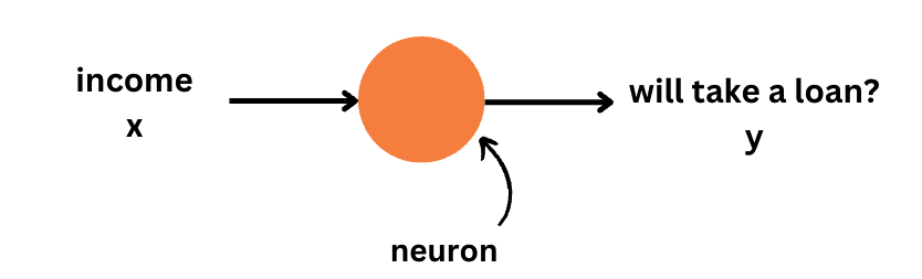
You already know how to do similar tasks using linear regression. A neuron is like a linear regression model with a few additional components. As in linear regression, a neuron takes an input (income), multiplies it by a weight, adds a bias, and generates an output. However, the neuron also includes an activation function, which introduces non-linearity to the output.
Activation Functions: Introducing Non-linearity
AActivation functions play a critical role in introducing non-linearity to the neuron's output. This is crucial because it allows the model to handle complex, non-linear data. A commonly used activation function is the Rectified Linear Unit (ReLU), which outputs the input value if it is positive and zero otherwise.
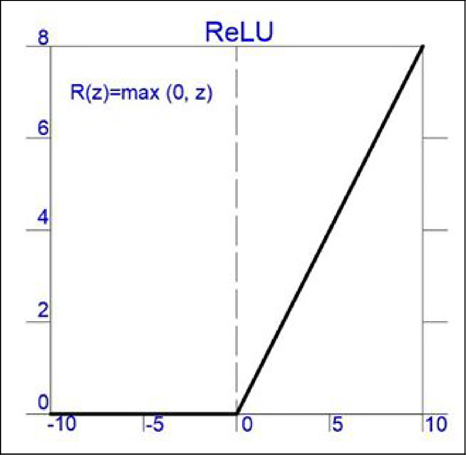
Constructing a Simple Neural Network
A neural network is essentially a series of neurons connected together. The output of one neuron feeds into the input of another. For example, in a simple network:
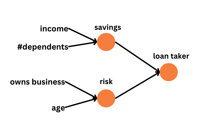
Deep Neural Networks: Beyond the Basics
When a neural network includes multiple layers of neurons, it becomes a deep neural network. These layers allow for the modeling of complex relationships and patterns in the data.
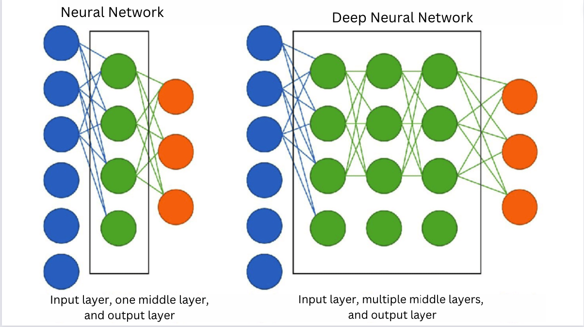
Watch the following video for a reiteration of the concepts we discussed above using a different example.
Coding a Neural Network Layer
To grasp the inner workings of neural networks, you can implement a layer in Python with just a few lines of code:
import numpy as np

class Layer:
    def __init__(self, input_size, output_size):
        self.weights = np.random.rand(input_size, output_size)
        self.bias = np.random.rand(output_size)

    def output(self, input):
        return np.dot(input, self.weights) + self.bias  # Linear operation plus bias
This simple example initializes a layer with random weights and biases, demonstrating how input is transformed through the layer.
[Optional] Here's an interesting video that demonstrates how to code a neural network layer from scratch using Python.
Note that the previous two examples don't involve learning. Learning, as we know, involves adjusting the weights and biases in a neural network to improve its performance. We will learn more about this in the next sections.
Neural Network Types
Neural networks come in various shapes and sizes, each designed to solve a specific problem. Watch the video below for a brief overview of the different types of neural networks:
Test Your Understanding
-
Q1. What is the difference between text, audio, and image data?
-
Q2. What are the use cases of a CNN (Convolutional Neural Network)?
-
Q3. What are the use cases of an RNN (Recurrent Neural Network)?
-
Q4. Which type of neural network is shown in the image below?
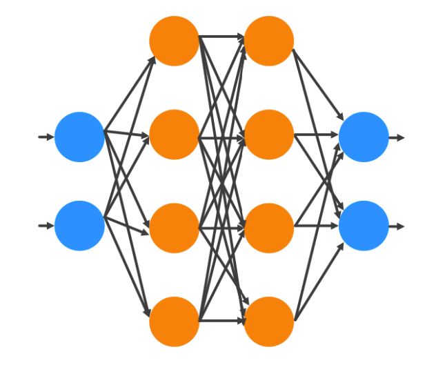
-
Q5. Which type of neural network is shown in the image below?
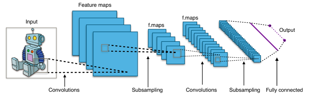
Practice Neural Networks
Follow the instructions in the neural networks practice notebook to build a neural network classifier for the MNIST dataset.

Computer Vision
Computer Vision is a transformative field within artificial intelligence that empowers computers and systems to extract meaningful information from digital images, videos, and other visual inputs. This field merges techniques from machine learning and traditional image processing to enable the interpretation and analysis of visual data.
Key Tasks in Computer Vision
Computer vision encompasses a range of tasks, each aimed at understanding visual data in some form. These include:
- Image Classification: Assigning a label to an image from a set of predefined categories.
- Object Detection: Identifying objects within an image and determining their boundaries.
- Image Segmentation: Dividing an image into segments to simplify its representation.
While machine learning algorithms, particularly those involving neural networks, play a crucial role in modern computer vision, the field also benefits from traditional image processing techniques. These foundational techniques, like filtering, edge detection, and image enhancement, are essential for preprocessing and improving image data for further analysis.
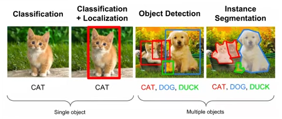
Basic Computer Vision Tasks: Berkeley CS198
Neural Networks in Computer Vision
Our exploration into neural networks revealed their potential in addressing computer vision challenges, such as image classification. However, standard neural networks face limitations in dealing with the complexity and scale of image data. This is due to their inability to efficiently handle large input sizes and to preserve the spatial structure of images (more on this later).
The Advent of Deep Learning in Computer Vision
Deep learning, a subset of machine learning, utilizes deep neural networks to uncover complex patterns in data. Its emergence has significantly advanced the field of computer vision, primarily through the use of Convolutional Neural Networks (CNNs). CNNs are adept at learning spatial hierarchies of features from images, making them particularly suited for computer vision tasks.
The breakthroughs in AI, particularly in computer vision, are largely attributed to the availability of large datasets and the computational capacity to train extensive models. The role of GPUs in this context cannot be overstated, as they have significantly accelerated the training processes.
Below is a comparison of some popular CNN architectures used in computer vision, including AlexNet, VGG, GoogLeNet, and ResNet. These models have been instrumental in advancing the field of computer vision, particularly in the ImageNet Large Scale Visual Recognition Challenge (ILSVRC).
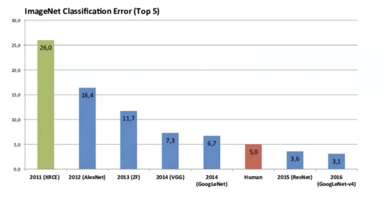
ImageNet Models Comparison: MIT6.S191
As we delve deeper into CNNs and their applications in computer vision, we'll explore how these models are constructed, trained, and utilized in various tasks, providing a deeper understanding of both deep learning and computer vision.
Convolutional Neural Networks (CNNs)
Convolutional Neural Networks (CNNs) stand as the cornerstone of deep learning applications in computer vision. Invented by Yann LeCun in the 1990s and continuously refined, CNNs excel in automatically learning spatial hierarchies of features from images. This capability has made them indispensable for a wide range of computer vision tasks, including image classification, object detection, and image segmentation.
Understanding CNNs is crucial for grasping the essence of deep learning and its application in analyzing visual data.
The Convolution Operation
At the heart of CNNs is the convolution operation, a specialized mathematical process that extracts features from input data using a kernel (or filter). This small matrix moves across the input data, applying a dot product at each step to produce a feature map, highlighting important features while reducing the size of the data.
The convolution operation transforms the input image in a manner that may seem almost magical, emphasizing features like edges and textures, which are vital for the subsequent layers of the CNN to build upon.


Convolution Operation
Watch this video to understand the convolution operation in more detail:
Understanding Feature Extraction in CNNs
Feature extraction in CNNs unfolds through the network's convolutional layers, which learn to identify features directly from the data. Initial layers might capture basic elements such as edges and corners, while deeper layers can discern more intricate details like textures and object parts. This hierarchical learning process enables CNNs to tackle complex visual recognition tasks effectively.
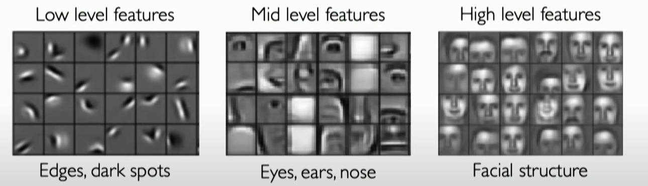
Watch this (trimmed) video to understand how CNNs learn features from data:
In our upcoming lessons, we'll dive into practical demonstrations of CNNs in action, showcasing their power in solving real-world computer vision challenges.
Building CNNs
Building CNNs involves stacking convolutional layers, pooling layers, and fully connected layers to create a deep learning model that can learn from visual data. Watch this video to understand how to build a Convolutional Neural Network (CNN):
Building CNNs in TensorFlow
TensorFlow is a popular deep learning framework that provides a high-level API for building and training CNNs. Watch this video to learn how to build a CNN in TensorFlow:
Extra Helpfull Resources
That concludes this lesson! You've explored the essential components of Convolutional Neural Networks and learned how to construct them with TensorFlow. In the upcoming lesson, we'll focus on the practical aspect of building image classifiers, specifically using the CIFAR-10 dataset.
CNN Layers
Convolutional Neural Networks (CNNs) are composed of various layers, each serving a distinct function and purpose. The most common layers found in CNNs include:
- Convolutional Layer
- Pooling Layer
- Fully Connected Layer
- Flatten Layer
- Dropout Layer
- Softmax Layer
Let's explore some of these layers in detail.
Pooling Layer
This layer reduces the spatial dimensions of the input feature map, thereby decreasing the computational load of the network and the risk of overfitting. Pooling operations, such as max pooling or average pooling, summarize the presence of features in patches of the feature map.
Watch the following video to understand the concept of pooling in CNNs:
Dropout Layer
The dropout layer is a regularization technique that randomly sets the outputs of several neurons in the layer to zero during training. This prevents the network from becoming too dependent on any single neuron and helps in reducing overfitting.
Watch the following video to understand the concept of dropout in CNNs:
Softmax Layer
The softmax layer is typically used in the final layer of a neural network-based classifier. It converts the outputs into probability distributions, making it easier to determine the target class.
Classic CNN Architectures
Over the years, a variety of CNN (Convolutional Neural Network) architectures have been developed, each contributing to advancements in the field of deep learning and its applications. Among these, some of the most renowned architectures include:
- LeNet-5: One of the earliest convolutional neural networks, pivotal for handwriting recognition.
- AlexNet: A breakthrough architecture that significantly outperformed competitors in the ImageNet challenge.
- VGGNet: Known for its simplicity and depth, with a focus on increasing the depth of the network using small filters.
- GoogLeNet : GoogLeNet: Introduced the inception module, enabling the network to choose from filters of various sizes.
- ResNet: Introduced residual connections to facilitate training of very deep networks, solving the vanishing gradient problem.
To better understand the unique architectures and contributions of these CNNs, watch the following video:
Practice CNN
Follow this Colab notebook to practice using CNNs. You will build a CNN model to classify images from the CIFAR-10 dataset.

Embark on a Historical Journey through Computer Vision and Neural Networks
Are you ready for a thrilling historical journey in the world of computer vision and neural networks?
In 2012, the field of computer vision was forever transformed by the introduction of AlexNet, a deep convolutional neural network that took the challenge of image recognition to unprecedented heights. Developed by Alex Krizhevsky, Ilya Sutskever, and Geoffrey Hinton, this groundbreaking model didn't just perform well—it shattered records, outperforming traditional methods by a staggering margin at the prestigious ImageNet Large Scale Visual Recognition Challenge (ILSVRC).
As you read through the paper, you'll gain insights into the architecture of convolutional neural networks (CNNs), understand the challenges the pioneers faced, and appreciate the elegant solutions they crafted. This isn't just a study session—it's an inspiration sprint. You'll see how embracing complexity and pushing boundaries in machine learning can lead to real-world impacts that were once thought to be in the realm of science fiction.
To start your journey, read the full paper here: AlexNet: ImageNet Classification with Deep Convolutional Neural Networks.
Week 6 Quiz : CNN
Before attempting the quiz, read the following carefully.
- This is a timed quiz. You will have one attempt.
- You will have 20 minutes to complete multiple-choice questions.
➡️ Access the quiz here.
Assignment: Face Recognition
In this assignment, you will build a face recognition model using a Convolutional Neural Network (CNN). You will use the ORL Faces dataset to train and test your model.
Please follow the instructions in the Colab notebook to complete the assignment. Some parts of the code are already implemented for you. You should write the code only where you are instructed to do so.

Submission
- Submit your notebook link via Gradescop here
Introduction to Logic and Knowledge Representation

Humans are logical beings. We use logic to reason about the world, and draw conclusions from facts. For example, if it’s sunny outside, we might decide to go for a walk. If it’s raining, we might decide to stay indoors. Can a computer do the same? Can a computer draw conclusions from facts and reason about the world?
We’ve seen how to achieve intelligence when we planned with search, modeled and used algebra with constraint satisfaction, learned from data with machine learning and deep learning, and learned by experience with reinforcement learning.
This week, we’ll explore how to achieve intelligence through logic and knowledge representation. We’ll start by understanding the basics of logic and knowledge representation, and then explore how to use logic to build intelligent systems. Let's start by asking the question: What is knowledge?
By the end of this lesson, you will be able to:
- Use propositional logic to represent facts and rules
- Use propositional logic to draw conclusions from facts and rules
- Use propositional logic to build an intelligent system like a medical diagnosis assistant
- Use first-order logic to represent more complex facts and rules utilizing quantifiers and predicates
Your assignment for this lesson is to build a home security system using propositional logic.
Logic and Knowledge Representation

What is logic?
In the context of AI, logic refers to a formal system used to represent and reason about knowledge and information. It is the same logic that we use in mathematics and philosophy, but applied to the domain of AI. Logic is used to represent facts and rules, and to draw conclusions from them. For example, we can use logic to represent the fact that "it's raining outside", and the rule that "if it's raining outside, then I should take an umbrella", and then use it to draw the conclusion that "I should take an umbrella".
What is Knowledge?
Knowledge refers to the information, understanding, and awareness that an individual or a system possesses about the world. It encompasses facts, concepts, beliefs, insights, experiences, and skills acquired through learning, observation, reasoning, and experimentation.
Knowledge of facts, also called propositional knowledge, is often characterized as true belief that is distinct from opinion or guesswork by virtue of justification. - Wikipedia
Since our study is about intelligent systems and decision making, we are interested in the propositional knowledge. This is the type of knowledge that can be represented as a set of propositions, or statements that can be either true or false.
Knowledge Representation (KB)
Knowledge representation is a field of artificial intelligence that focuses on how to formally represent knowledge in a way that can be used to solve problems.
Based on the goals and the type of questions you will ask or use the KB for, you would select the appropriate knowledge representation model. For example, if you are interested in representing the knowledge in a way that allows you to query facts, you would use a different model than if you are interested in representing the knowledge in a way that allows you to generate new content.
Knowledge Representation Models
Semantic Networks, Frames, Conceptual Graphs, Neural Networks and Logic are all examples of knowledge representation models. Each model is suitable for different types of problems.
Semantic networks, for example, are suitable for representing knowledge about the relationships between objects, which is useful in building cognitive systems like chatbots. On the other hand, logic-based knowledge representation is suitable for representing facts and rules, which is useful in building expert systems.
In this lesson, we focus on the logic-based knowledge representation model. This model allows us to represent facts and rules, and to draw conclusions from them.
An example of what we can do with logic-based knowledge representation is a medical diagnosis assistant.
-
If a person exhibits sneezing and a runny nose but no fever, it is certain that they have allergies.
-
If a person exhibits fever, cough, and body aches, it is certain that they have flu.
-
If a person exhibits cough and runny nose, but no fever, it is certain that they have a common cold.
We can represent these facts and rules in a knowledge base, using propositional logic or first-order logic, and then use it to diagnose a patient based on their symptoms.
Different Types of Logic
There are different types of logic, each suitable for different types of problems. The two main types of logic that we will focus on in this class are:
- Propositional Logic
- First-Order Logic
Other types of logic include:
- Temporal Logic
- Fuzzy Logic
- Probabilistic Logic
- and more.
Propositional Logic
Propositional logic is a type of logic that deals with propositions. A proposition is a statement that is either true or false. For example, "Kibo is an institution that allows students to earn a degree in Computer Science." is a proposition, and it is true. "The sky is green" is also a proposition, but it is false.
Propositional Symbols
In propositional logic, we use variables (or symbols) to represent propositions. For example, we can use the variable p to represent the proposition "Kibo is an institution that allows students to earn a degree in Computer Science." and the variable q to represent the proposition "The sky is green". We can then use logical operators to combine these propositions.
Premises
In logic, the term "premises" refers to the statements or propositions that are assumed to be true in an argument or inference.
Sentences
A sentence is a combination of propositions and logical operators. For example, the sentence "The sky is blue and it is daytime" is a combination of the propositions "The sky is blue" and "It is daytime" using the logical operator "and".
Logical Connectives
Logical connectives are operators that can be used to combine propositions. The main logical connectives are:
-
Negation or Not (¬): This operator takes a proposition and returns its negation. For example, if p is the proposition "The sky is blue", then ¬p is the proposition "The sky is not blue".
-
Conjunction or And (∧): This operator takes two propositions and returns their conjunction. For example, if p is the proposition "The sky is blue" and q is the proposition "It is daytime", then p ∧ q is the proposition "The sky is blue and it is daytime".
-
Disjunction or Or (∨): This operator takes two propositions and returns their disjunction. For example, if p is the proposition "The sky is blue" and q is the proposition "The sky is green", then p ∨ q is the proposition "The sky is blue or the sky is green".
-
Implication (→): This operator takes two propositions and returns their implication (if...then). For example, if p is the proposition "The sky is blue" and q is the proposition "It is daytime", then p → q is the proposition "If the sky is blue, then it is daytime".
-
Biconditional (↔): This operator takes two propositions and returns their biconditional. For example, if p is the proposition "The sky is blue" and q is the proposition "The sky is green", then p ↔ q is the proposition "The sky is blue if and only if the sky is green".
Truth Tables
Truth tables are tables that show the truth value of a compound proposition for all possible combinations of truth values of its components. For example, the truth table for the conjunction p ∧ q is:
| p | q | p ∧ q |
|---|---|---|
| True | True | True |
| True | False | False |
| False | True | False |
| False | False | False |
The truth table for the implication p → q is:
| p | q | p → q |
|---|---|---|
| True | True | True |
| True | False | False |
| False | True | True |
| False | False | True |
The truth table for the biconditional p ↔ q is:
| p | q | p ↔ q |
|---|---|---|
| True | True | True |
| True | False | False |
| False | True | False |
| False | False | True |
Knowledge Base (KB)
In the context of propositional logic, A knowledge base is a set of propositions that represent the facts and rules about the world. For example, the knowledge base for the medical diagnosis assistant we mentioned earlier might contain the following proposition:
"If a person exhibits sneezing and a runny nose but no fever, it is certain that they have allergies."
Which can be represented as: ( S ^ R ^ ¬F ) → A
Where:
- S: A person has sneezing.
- R: A person has a runny nose.
- F: A person has fever.
- A: A person has allergies.
It represents the rule that if a person has sneezing and a runny nose, but no fever, then they have allergies.
You can write a simple python code to represent the above knowledge base and query it just by using if else statements. However, in real-world problems, the knowledge base can be very large and complex, and so it is not practical to use if else statements to represent it. This is where logic-based knowledge representation comes in handy.
Representing the facts and the rules, as we did above, is a cruical step in building an intelligent system that can reason about the world. The next step will be using algorithms to draw conclusions from the knowledge base.
Watch this video for another example:
Code Example
Let's write a simple python code to represent the medical diagnosis knowledge base we mentioned earlier and query it.
# colab notebook for this code is available here:
# https://colab.research.google.com/drive/1DQMAZz8j_-OeZ932crsQE3hIukBFBSr2

# Define symbols
S = Symbol("Sneezing")
R = Symbol("RunnyNose")
F = Symbol("Fever")
A = Symbol("Allergies")


# Construct the knowledge base
knowledge = Implication(And(S, R, Not(F)), A)

# a set of propositions that represent a possible state about the world that we can query next
model = And(And(S, R), Not(F))

# query to ask
query = Implication(model, A)

# Check if the knowledge base entails the person has allergies
# can we imply A (Allergies) from the model ( S ^ R ^ ¬F )?
result = model_check(knowledge, query)

print("Does the person have allergies?", result)
In the above code, we define the symbols S, R, F, and A to represent the propositions "A person has sneezing", "A person has a runny nose", "A person has fever", and "A person might have allergies", respectively.
We then construct the query to represent the question "Does the person have allergies if they have sneezing and a runny nose, but no fever?".
The code used the model_check function to check if the knowledge base entails the query. We will discuss the model_check function in the next section.
Entailment
The result of the above program is True, which means that the knowledge base entails the query, and so the person has allergies.
Entailment is the relationship between a knowledge base and a query. A knowledge base entails a query if the query is true in the knowledge base.
The notation for entailment is |=. For example, if KB is the knowledge base and q is the query, then KB |= q means that the knowledge base entails the query.
Test Your Understanding
Q1. In the context of a knowledge base (KB) in propositional logic, what does the expression (S ∧ R ∧ ¬F) → A signify given the propositions S: Sneezing, R: Runny Nose, F: Fever, A: Allergies?
- A) If a person has sneezing, a runny nose, and no fever, then they have allergies.
- B) A person with a fever, sneezing, and a runny nose has allergies.
- C) Sneezing and a runny nose are sufficient to conclude allergies, regardless of fever.
- D) If a person has allergies, they will have sneezing, a runny nose, and no fever.
Q2. Consider the propositions p: "The sky is blue", q: "It is raining". Which of the following represents the statement "If the sky is blue, then it is raining"?
- A) p → q
- B) p ∧ q
- C) p ∨ q
- D) p ↔ q
Consider the propositions p: "The sky is blue", q: "It is raining". Which of the following represents the biconditional 'p if and only if q'?
- A) p → q
- B) p ∧ q
- C) p ∨ q
- D) p ↔ q
Answer
Q1. The correct answer is A) If a person has sneezing, a runny nose, and no fever, then they have allergies.Q2. The correct answer is A) p → q
Q3. The correct answer is D) p ↔ q
Summary
- Propositional logic is a type of logic that deals with propositions.
- A proposition is a statement that is either true or false.
- Propositional logic uses variables (or symbols) to represent propositions.
- Logical connectives are operators that can be used to combine propositions.
- A knowledge base is a set of propositions that represent the facts and rules about the world.
- Entailment is the relationship between a knowledge base and a query. A knowledge base entails a query if the query is true in the knowledge base.
Practice: KB Representation
Open the Colab notebook below and complete the following exercise:
Extend the knowledge base in the notebook to include the following two rules:
-
If a person exhibits fever, cough, and body aches, it is certain that they have the flu.
-
If a person exhibits cough and a runny nose, but no fever, it is certain that they have a common cold.

Possible Solution
# Define symbols
S = Symbol("Sneezing")
R = Symbol("RunnyNose")
F = Symbol("Fever")
A = Symbol("Allergies")
C = Symbol("Cough")
B = Symbol("BodyAches")

# Construct the knowledge base
knowledge = And(
    Implication(And(S, R, Not(F)), A),  # Rule for allergies
    Implication(And(F, C, B), Symbol("Flu")),  # Rule for flu
    Implication(And(C, R, Not(F)), Symbol("CommonCold"))  # Rule for common cold
)

# Questions
questions = [
    (And(F, C), "Does the person have a common cold?"),  # Question 1
    (And(F, B, C), "Does the person have a common cold?"),  # Question 2
    # Add more questions here
]

# Check each question against the knowledge base
for query, question_text in questions:
    result = model_check(knowledge, query)
    print(question_text, result)
Inferring with Logic
Inference is the process of determining whether a given sentence can be derived from the knowledge base.
Assume a knowledge base with the following formulae:
KB = ( A ∨ C ) ∧ (B ∨ ¬ C )
It could be representing something like:
- A: It is raining.
- B: It is cloudy.
- C: You have an umbrella.
And the knowledge base states that "It is raining or you have an umbrella" and "It is cloudy or you don't have an umbrella".
KB = ( A ∨ C ) ∧ (B ∨ ¬ C )
Our aim is to determine if the sentence α = ( A ∨ B ) can be inferred from the knowledge base or not.
To solve similar problems, we need an inference algorithm. An inference algorithm is a procedure to determine whether a given sentence can be derived from the knowledge base.
There are several algorithms to perform inference in propositional logic. Some of the most common algorithms are:
- Truth Table
- Forward Chaining
- Backward Chaining
- Resolution
Model Checking with Truth Table
The model checking approach uses truth tables for inference. It is a brute force algorithm that checks all possible interpretations of the knowledge base. The algorithm works as follows:
-
Create a truth table with all possible combinations of truth values for the propositional symbols in the knowledge base.
-
For each interpretation, check if the knowledge base entails the sentence α (i.e. sentence α evaluates to true whenever KB evaluates to true)
| A | B | C | A ∨ C | (B ∨ ¬C) | KB | α |
|---|---|---|---|---|---|---|
| True | True | True | True | True | True | True |
| True | True | False | True | True | True | True |
| True | False | True | True | False | False | True |
| True | False | False | True | True | True | True |
| False | True | True | True | True | True | True |
| False | True | False | False | True | False | True |
| False | False | True | True | False | False | False |
| False | False | False | False | True | False | False |
We have 3 symbols (A, B, C), so we have 2^3 = 8 possible interpretations. For all possible interpretations, The sentence α evaluates to true whenever the knowledge base evaluates to true. Therefore, we can conclude that the sentence α can be inferred from the knowledge base.
In logic.py module that we used earlier, this is what the function model_check does. It enumerates all possible interpretations and checks if the knowledge base entails a given sentence or not.
Inferring with Model Checking
Watch the video (~20 minutes) below to see an example of the model checking algorithm.
The video shows how to use the model checking algorithm to determine if a given sentence can be inferred from the knowledge base.
The code used in the video is available here
Soundness and Completeness
Soundness
A logical inference algorithm is said to be sound if it never derives a false conclusion from premises. In other words, it will not give wrong answers (false positives).
The truth model checking approach is a sound algorithm. It does not give us wrong answers.
Completeness
An inference algorithm is complete if it is capable of deriving any valid conclusion that can be drawn from a given set of premises. In other words, it checks all possible interpretations and does not miss any valid inference.
The model checking approach is a complete algorithm. It checks all possible interpretations and does not miss any valid inference.
Question:
What is the time complexity of the model checking / truth table algorithm?
Think about the number of rows in the truth table and the number of propositional symbols in the knowledge base. Think about it before you click to see the answer below.
Click to see the answer
The truth table approach has an exponential time complexity. It requires 2n rows in the truth table, where n is the number of propositional symbols in the knowledge base. Therefore, the truth table approach is not practical for large knowledge bases.Inference Rules
As we need only to check the KB for True values, we can improve the truth table algorithm by using the inference rules approach. We can use the inference rules to simplify the knowledge base and then check if a sentence α can be inferred from the simplified knowledge base. Inference rules can be used to generate new (sound) sentences from existing ones.
Inference Rules
Inference rules are used to generate new sentences from existing ones. Some of the most common inference rules are:
-
Modus Ponens: If we know that
AimpliesBand we know thatAis true, then we can infer thatBis true. -
And Elimination: If we know that
A ∧ Bis true, then we can infer thatAis true and we can infer thatBis true. -
Double Negation: If we know that
Ais true, then we can infer that¬¬Ais true. -
Implication Elimination: If we know that
AimpliesB, then we can infer that¬A ∨ Bis true. -
Bidirectional Elimination: If we know that
Ais true if and only ifBis true, then we can infer that(A → B) ∧ (B → A)is true. -
De Morgan's Law: If we know that
¬(A ∧ B)is true, then we can infer that¬A ∨ ¬Bis true. -
Distribution: If we know that
A ∨ (B ∧ C)is true, then we can infer that(A ∨ B) ∧ (A ∨ C)is true. -
And many more...
[Optional] Inference By Resolution
Inferring by resolution is based on the resolution rule, which is a sound and complete inference rule. The resolution rule is used to generate new clauses from existing ones.
Watch the video below to see how to use the resolution rule to perform inference.
Summary
- Inference is the process of determining whether a given sentence can be derived from the knowledge base.
- The model checking approach uses truth tables for inference. It is a sound and complete algorithm, but it has an exponential time complexity.
- Inference rules can be used to simplify the knowledge base and then check if a sentence
αcan be inferred from the simplified knowledge base. - The resolution rule is a sound and complete inference rule. It is used to generate new clauses from existing ones.
First Order Logic
First Order Logic is a type of logic that extends propositional logic by allowing us to represent more complex statements and reason about them. In first order logic, we can use quantifiers to express statements about objects and predicates to express relationships between objects.
Constant Symbols
In first order logic, a constant is a symbol that represents a specific object in a domain. For example, we can use the constant Solomon to represent the object 'Solomon' and the constant Math to represent the subject 'Math'.
Predicate Symbols
In first order logic, a predicate symbolically represents a property or relationship that can be true or false for objects. It takes objects as arguments. For example, we can use the predicate Student(x) to represent the statement "x is a student". Another example is the predicate TakesCourse(x, y) which represents the statement "x takes the course y".
Examples of predicate symbols:
Student(Solomon): This predicate indicates that 'Solomon' is a student.TakesCourse(Solomon, Math): This predicate indicates that 'Solomon' takes the course 'Math'.¬TakesCourse(Solomon, JavaEE): This predicate indicates that 'Solomon' does not take the course 'JavaEE'.
Quantifiers
Quantifiers are used to express more complex statements about objects. The two main quantifiers in first order logic are:
-
Universal Quantifier (∀): This quantifier is used to express that a statement is true for all objects in a domain. For example, the statement 'All students take Prog1 class' can be expressed as:
∀x Student(x) → TakesCourse(x, Prog1). -
Existential Quantifier (∃): This quantifier is used to express that a statement is true for at least one object in a domain. For example, the statement 'Some students take JavaEE class' can be expressed as:
∃x Student(x) ∧ TakesCourse(x, JavaEE).
Logic Programming : A New Programming Paradigm
First order logic is the foundation of logic programming, a programming paradigm that uses logical inference to solve problems. In logic programming, we can use first order logic to represent the rules and facts about a problem, and then use a logical inference engine to derive new facts and solve problems.
The most popular logic programming language is Prolog, which is based on first order logic and is used in artificial intelligence and natural language processing.
Logic programming is a general-purpose programming paradigm that can be used to solve a wide range of problems, including constraint satisfaction problems, planning problems, and natural language processing problems.
Here is an example of a Prolog program that uses first order logic to represent the rules and facts about courses, students, and professors:
studies(charlie, csc135).
studies(olivia, csc135).
studies(jack, csc131).
studies(arthur, csc134).

teaches(kirke, csc135).
teaches(collins, csc131).
teaches(collins, csc171).
teaches(juniper, csc134).


professor(X, Y) :-
    teaches(X, C), studies(Y, C).

## Queries
?- studies(charlie, What). // charlie studies what? OR What does charlie study?
?- professor(kirke, Students). // Who are the students of professor kirke.
Here is a sample run output from Online SWI-Prolog Interpreter

An extensive discussion on Logic Programming is beyond the scope of this class but it is important to know about it and be able to identify potential uses of logic programming in your engineering career.
Summary
- First order logic extends propositional logic by allowing us to represent more complex statements and reason about them.
- In first order logic, we can use constant symbols to represent specific objects in a domain, predicate symbols to represent relationships between objects, and quantifiers to express more complex statements about objects.
- The two main quantifiers in first order logic are the universal quantifier (∀) and the existential quantifier (∃).
- The universal quantifier is used to express that a statement is true for all objects in a domain, while the existential quantifier is used to express that a statement is true for at least one object in a domain.
Practice: First Order Logic
Q1. Translate the statement "David is a professor." into First-Order Logic.
Answer
Professor(David)Q2. Translate the statement "Mohammed Teaches AI." into First-Order Logic.
Answer
Teaches(Mohammed, AI)Q3. Translate the statement "Deans are professors." into First-Order Logic.
Answer
∀x (Dean(x) → Professor(x))Convert the sentence "There exists a product with a price higher than $100" into First-Order Logic.
Answer
∃x (Product(x) ∧ Price(x) > 100)Translate the statement "For every product that has been ordered, there exists a customer who placed the order" into First-Order Logic.
Answer
∀x (Product(x) ∧ Ordered(x) → ∃y (Customer(y) ∧ PlacedOrder(y, x)))Represent the statement "All employees who work on a project are assigned specific tasks" in First-Order Logic.
Answer
∀x (Employee(x) ∧ WorksOnProject(x) → ∃y (Task(y) ∧ AssignedToTask(x, y)))Week 7 Quiz
Before attempting the quiz, read the following carefully.
- This is a timed quiz. You will have only one attempt.
- You will have 20 minutes to complete multiple-choice questions.
➡️ Access the quiz here.
Assignment: Home Security System
The objective of this assignment is to use propositional logic to model and query a basic security system for a home. The home is equipped with various sensors and alarms, and the system should be capable of answering queries about the home's state.
➡️ Access the assignment and all details here.
Introduction to NLP

This image was generated with the help of Natural Language Processing (NLP).
Ever wondered how chatbots, such as ChatGPT, can feel so remarkably human-like in their responses? Or marveled at how your favorite virtual assistant always seems to know just what you need? Get ready to uncover the exciting secrets behind language translation, text summarization, question answering, text classification, and much more! Welcome to the world of Natural Language Processing (NLP)! It's the groundbreaking technology that makes all of this possible.
Natural Language Processing (NLP) is a field of computer science, artificial intelligence, and computational linguistics. It focuses on the interactions between computers and human (natural) languages.
When we discussed computer vision, we learned that its aim is to empower computers to comprehend, analyze, and effectively utilize visual information. Similarly, NLP serves the same purpose but for textual data. It involves the capability of a computer program to understand human language as it is spoken or written.
After completing this lesson, you will be able to:
- Explain what Natural Language Processing (NLP) is.
- Clean text data.
- Perform basic NLP tasks such as tokenization, stemming, and lemmatization.
- Explain Language Models and their applications.
- Build NLP applications such as sentiment analysis, text summarization, and text generation.
Language and Natural Language Processing

Let's start by defining what a language is and what is natural language processing.
A language is a system of communication that is used to express thoughts, feelings, and ideas. It is a system that is made up of words, grammar, and syntax.
A Natural Language, such as English, is a language that has evolved naturally in human societies. It is a language that is spoken and written by humans.
An artificial language, like Python, is a language that has been designed by humans for a specific purpose. For example, Python is a language that has been designed for computer programming.
Processing, In computing, 'processing' refers to the methods and techniques used by computers to handle tasks such as understanding, generating, and translating human language.
Natural Language Processing (NLP) is the study of how computers can deal with human language. For example, understanding the purpose of a text, generate a summary of a text, or translate a text from one language to another.
Natural Language Complexity
Natural languages, unlike artificial ones, are inherently complex, presenting numerous challenges for computer comprehension. This complexity arises from various factors, including the ambiguity of human language, the contextual nuances within which text is employed, and the requisite background knowledge necessary for understanding.
Here is an article that delves deeper into the reasons why natural languages are difficult: Why Human Language is Hard
NLP has existed for more than 50 years, but it has gained significant traction in the last decade due to the rise of deep learning and the availability of large-scale datasets. It has roots and close ties to the field of linguistics.
In the 1950s, with the aspiration for machine translation, encountering early setbacks that led to the first AI Winter. By the 1960s, the field experienced a revival with innovations such as ELIZA, an early chatbot. The late 1990s witnessed a paradigm shift towards statistical models, leveraging data over predefined rules.
Applications of NLP
1. Text Classification
Text classification involves categorizing text documents into predefined categories or classes. NLP techniques are used to analyze the content of text documents and assign appropriate labels based on their topics, sentiments, or other attributes. Applications include spam detection, sentiment analysis, topic modeling, and content categorization.
2. Machine Translation
Machine translation aims to automatically translate text from one language to another. NLP models are trained on large bilingual corpora to learn the mappings between languages and generate accurate translations. Popular examples include Google Translate, Microsoft Translator, and DeepL.
3. Named Entity Recognition (NER)
Named Entity Recognition (NER) is the task of identifying and classifying named entities (such as persons, organizations, locations, and dates) in text data. NLP techniques are used to extract and classify entities, which is essential for various applications such as information extraction, question answering systems, and entity linking.
4. Text Summarization
Text summarization involves condensing large volumes of text into shorter, coherent summaries while retaining the most important information. NLP techniques, including extractive and abstractive summarization methods, are employed to generate concise and informative summaries from documents, articles, or other textual content.
5. Sentiment Analysis
Sentiment analysis, also known as opinion mining, aims to determine the sentiment or emotional tone expressed in a piece of text. NLP models analyze the text to classify it as positive, negative, or neutral, providing valuable insights into public opinion, customer feedback, and social media sentiment.
6. Question Answering Systems
Question Answering (QA) systems automatically generate accurate answers to user queries posed in natural language. NLP techniques, combined with information retrieval and knowledge representation methods, enable QA systems to understand questions, search for relevant information, and generate appropriate responses from structured or unstructured data sources.
And many more! NLP has a wide range of applications across various domains, including healthcare, finance, e-commerce, education, and entertainment.
Cleaning
Before we can start building NLP models or executing NLP tasks, we need to clean the text. This is important because it ensures that the text is consistent and that the model can learn from it effectively.
The list of cleaning approaches is long and depends on the specific task and the data. Some typical cleaning approaches include removing punctuation, converting text to lowercase, removing stop words, removing special characters, and many more. Most of these cleaning approaches can be implemented using regular expressions and basic Python's string methods. However, some cleaning tasks may require more complex methods.
Let's explore some common cleaning approaches further.
Removing Stop Words
To remove stop words, we need to first download the list of stop words from the NLTK library. Then, we can remove the stop words from the text using a list comprehension.
import nltk
from nltk.corpus import stopwords

# Removing stop words
stop_words = set(stopwords.words('english'))
text = "the quick brown fox jumps over the lazy dog"

text = ' '.join([word for word in text.split() if word not in stop_words])

print(text) # quick brown fox jumps lazy dog
Lemmatization
A lemma is the base form of a word. For instance, the lemma of "rocks" is "rock". Lemmatization is the process of reducing words to their base or root form. This is important because it ensures that the model treats words with different forms consistently. Lemmatization involves determining the base or dictionary form of a word based on its context. It uses language dictionaries and morphological analysis to accurately reduce words to their base form.
To lemmatize the text, we can use the WordNetLemmatizer from the NLTK library.
import nltk
from nltk.stem import PorterStemmer, WordNetLemmatizer
nltk.download('wordnet')

text = "rocks and cats"

lemmatizer = WordNetLemmatizer()
text = ' '.join([lemmatizer.lemmatize(word) for word in text.split()])
print(text) # rock and cat
Stemming
Stemming performs a similar function to lemmatization. It follows a rule-based approach reduces words to 1their base or root form by removing suffixes, such as "ing" or "ed".
import nltk
from nltk.stem import PorterStemmer, WordNetLemmatizer
nltk.download('wordnet')

text = "running in a stunning day"

stemmer = PorterStemmer()
text = ' '.join([stemmer.stem(word) for word in text.split()])

print(text) # run in stun day
Note that the NLTK's WordNetLemmatizer is designed to lemmatize words based on their part-of-speech (POS) tag. By default, if no POS tag is specified, it assumes the word is a noun. However, to lemmatize verbs accurately, you need to explicitly provide the POS tag.
lemmatizer.lemmatize("runnin") # running
lemmatizer.lemmatize("running", pos = 'v') # run
Exercise
Use any paragraph of text and clean it using the following steps:
- Remove punctuation marks.
- Convert all text to lowercase.
- Remove numbers.
- Remove stopwords (common words that often do not carry significant meaning like "the", "is", "and", etc.).
Tokenization
Probably the first thing most NLP algorithms have to do is to split the text into tokens, this is called tokenization. Tokenization is the process of breaking a text into words, phrases, symbols, or other meaningful elements.
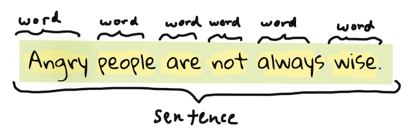
Tokenizing a sentence from Pride and Prejudice. Infographic by Jen Looper
You've probably built some tokenizers yourself, even if you didn't realize it. For example, if you've ever used the split method in Python, you've tokenized a string. However, tokenization is not always as simple as splitting a string by spaces. For example, in the sentence "Good muffins cost $3.88 in New York. Please buy me... two of them.\n\nThanks.", the ellipsis ("..."), the dollar sign ("$"), and the newline characters ("\n") are all tokens that should be separated from the words.
Luckily, there are many libraries that provide tokenization methods that can handle these edge cases. Natural Language Toolkit (nltk) library provides a word_tokenize method that can handle these edge cases. Here's an example of how to use it:
# pip install nltk to install nltk

from nltk.tokenize import word_tokenize
text = "Good muffins cost $3.88\nin New York.  Please buy me... two of them.\n\nThanks."
tokens = word_tokenize(text)
print(tokens)
This code will output:
['Good', 'muffins', 'cost', '$', '3.88', 'in', 'New', 'York', '.', 'Please', 'buy', 'me', '...', 'two', 'of', 'them', '.', 'Thanks', '.']
The library spaCy also provides a tokenizer that can handle these edge cases. Here's an example of how to use it:
# pip install spacy # to install the spacy
# spacy download en_core_web_sm # to download the english model

import spacy
nlp = spacy.load("en_core_web_sm")
doc = nlp("Good muffins cost $3.88\nin New York.  Please buy me... two of them.\n\nThanks.")
tokens = [token.text for token in doc]
print(tokens)
This code will output:
['Good', 'muffins', 'cost', '$', '3.88', '\n', 'in', 'New', 'York', '.', ' ', 'Please', 'buy', 'me', '...', 'two', 'of', 'them', '.', '\n\n', 'Thanks', '.']
The sent_tokenize method in nltk and spaCy can be used to tokenize sentences. Here's an example of how to use it in nltk:
from nltk.tokenize import sent_tokenize
text = "Good muffins cost $3.88\nin New York.  Please buy me... two of them.\n\nThanks."
sentences = sent_tokenize(text)
print(sentences)
This code will output:
['Good muffins cost $3.88\nin New York.', 'Please buy me... two of them.', 'Thanks.']
And here's an example of how to use it in spaCy:
import spacy
nlp = spacy.load("en_core_web_sm")
doc = nlp("Good muffins cost $3.88\nin New York.  Please buy me... two of them.\n\nThanks.")
sentences = [sent.text for sent in doc.sents]
print(sentences)
This code will output:
['Good muffins cost $3.88\nin New York.', 'Please buy me... two of them.', 'Thanks.']
Keras also provides a tokenizer that can be used to tokenize text. Here's an example of how to use it:
from keras.preprocessing.text import Tokenizer

# Example text data
texts = [
    "This is an example sentence.",
    "Another example sentence to tokenize."
]

# Initialize tokenizer
tokenizer = Tokenizer()

# Fit tokenizer on texts
tokenizer.fit_on_texts(texts)

# Convert texts to sequences of tokens
sequences = tokenizer.texts_to_sequences(texts)

# Print tokenized sequences
print("Tokenized sequences:")
for seq in sequences:
    print(seq)
The output of this code will be:
Tokenized sequences:
[3, 4, 5, 1, 2]
[6, 1, 2, 7, 8]
This code initializes a Keras Tokenizer, fits it on the example texts, and then converts the texts into sequences of tokens. Additionally, it builds a word index that can be used to convert tokens back into words. Finally, it prints the tokenized sequences.
Here's an example of how to use the word index to convert tokens back into words:
# Convert tokens back into words
print("Words:")
word_index = tokenizer.word_index
for seq in sequences:
    words = [list(word_index.keys())[list(word_index.values()).index(word_id)] for word_id in seq]
    print(" ".join(words))
Different Tokenization Approaches
Besides the word and sentence tokenization, there are other tokenization approaches that are used in NLP, such as:
-
Subword Tokenization: This approach splits words into smaller units, such as characters or subwords. This is useful for languages like Turkish, where words can be very long and complex. It is also useful for languages like English, where words can be combined to form new words, such as "unbelievable" and "incredible".
-
Byte Pair Encoding (BPE): This is a subword tokenization approach that is used in many NLP models such as GPT-2 and GPT-3. It is based on the frequency of pairs of characters in a corpus of text.
-
WordPiece Tokenization: This is a subword tokenization approach that is used in many NLP models, such as BERT. It is based on the frequency of words in a corpus of text. It is useful for languages like English, where words can be combined to form new words, such as "unbelievable" and "incredible".
-
Character Tokenization: This approach splits words into characters. This is useful for languages like Chinese, where there are no spaces between words.
-
And more...
N-grams
N-grams are sequences of n words. For example, "I am" is a 2-gram (or bigram), "I am learning" is a 3-gram (or trigram), and "I am learning NLP" is a 4-gram (or 4-gram). N-grams are used in many NLP tasks, such as language modeling, machine translation, and text generation.
N-grams. Infographic by Jen Looper
We can consider that N-grams are sequences of the tokens we generated in the tokenization process. For example, if we have the sentence "I am learning NLP", the 2-grams (or bigrams) would be "I am", "am learning", and "learning NLP". The 3-grams (or trigrams) would be "I am learning" and "am learning NLP". And the 4-grams would be "I am learning NLP".
You can use the ngrams method in the nltk library to generate n-grams. Here's an example of how to use it:
import nltk
from nltk.util import ngrams

# Example sentence
sentence = "The quick brown fox jumps over the lazy dog."

nltk.download("punkt")

# Tokenize the sentence
tokens = nltk.word_tokenize(sentence)

# Generate n-grams
n = 2  # Example for bigrams
bigrams = list(ngrams(tokens, n))

# Print the bigrams
print("Bigrams:", bigrams)
This code will output:
[nltk_data] Downloading package punkt to /root/nltk_data...
[nltk_data]   Unzipping tokenizers/punkt.zip.

Bigrams: [('The', 'quick'), ('quick', 'brown'), ('brown', 'fox'), ('fox', 'jumps'), ('jumps', 'over'), ('over', 'the'), ('the', 'lazy'), ('lazy', 'dog'), ('dog', '.')]
N-grams play pivotal roles across various NLP tasks, including language modeling, machine translation, and text generation. Moreover, they are integral components within numerous NLP models, exemplified by GPT-2 and BERT.
Part-of-Speech Tagging
Every word that has been tokenized can be tagged as a part of speech - a noun, verb, or adjective. The sentence "the quick red fox jumped over the lazy brown dog" might be POS tagged as fox = noun, jumped = verb.
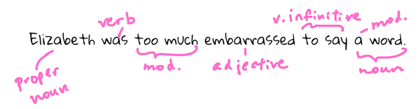
POS tagging a sentence from Pride and Prejudice. Infographic by Jen Looper
In information retrieval and search engines, part-of-speech tagging (POS tagging) helps in improving search engine results by understanding the context of search queries. For example, distinguishing between nouns and verbs can help prioritize search results based on the user's intent. It could also be used in other NLP tasks, such as named entity recognition, text classification, and sentiment analysis.
You can use the pos_tag method in the nltk library to POS tag a sentence. Here's an example of how to use it:
import nltk
from nltk.tokenize import word_tokenize

# Sample sentence
sentence = "The quick brown fox jumps over the lazy dog."

# Tokenize the sentence
tokens = word_tokenize(sentence)

# Perform POS tagging
pos_tags = nltk.pos_tag(tokens)

# Print the POS tags
print("POS tags:")
print(pos_tags)
Named Entity Recognition
Named Entity Recognition (NER) is the process of identifying and classifying named entities in a text. Named entities are real-world objects such as persons, locations, organizations, dates, and more. NER is a fundamental task in information extraction and text analysis, and it is used in a wide range of applications such as question answering, information retrieval, and machine translation.
NER can be used to extract structured information from unstructured text data. For example, in the sentence "Apple is headquartered in Cupertino, California", NER can be used to identify "Apple" as an organization and "Cupertino, California" as a location.
Example:
import nltk

# Sample text
text = """
Barack Obama was born in Hawaii. He served as the 44th President of the United States from 2009 to 2017.
"""

# Tokenize the text into sentences
sentences = nltk.sent_tokenize(text)

# Tokenize each sentence into words and perform part-of-speech tagging
tagged_sentences = [nltk.pos_tag(nltk.word_tokenize(sentence)) for sentence in sentences]

# Perform named entity recognition (NER)
named_entities = nltk.ne_chunk_sents(tagged_sentences, binary=False)

# Function to extract named entities from the named entity chunk tree
def extract_entities(tree):
    entities = []
    if hasattr(tree, 'label') and tree.label():
        if tree.label() == 'NE':
            entities.append(' '.join([child[0] for child in tree]))
        else:
            for child in tree:
                entities.extend(extract_entities(child))
    return entities

# Extract named entities from each chunk tree
named_entities_list = []
for tree in named_entities:
    for entity in extract_entities(tree):
        named_entities_list.append(entity)

# Print named entities
print("Named Entities:")
for entity in named_entities_list:
    print(entity)
Text Segmentation
Before we tokenize a text, specifically a long text, we might need to segment it into paragraphs, sections, or other meaningful units. This is called text segmentation.
Text segmentation is the process of dividing a text into meaningful units, such as paragraphs, sections, or chapters.
This process could be as simple as splitting a text by newline characters or as complex as using machine learning algorithms to identify the boundaries of paragraphs or sections. It's important to note that nltk and spaCy` do not provide built-in methods for segmenting text into paragraphs or sections.
Exercises
Open a python file in your local dev environment, install the required libraries, and complete the following exercises.
-
Exercise 1: Tokenize the following sentence using the
word_tokenizemethod innltk: "Welcome to your professional community" -
Exercise 2: Tokenize the following sentence using the spaCy tokenizer: "Welcome to your professional community"
-
Exercise 3: Generate bigrams for the following sentence: "While spaCy can be used to power conversational applications, it’s not designed specifically for chat bots, and only provides the underlying text processing capabilities.".
Word Representation
To make our job easier while working with text on a computer, we need to represent words in a way that will help us solve a certain task, such as text classification or named entity recognition. In this lesson, we will discuss different ways to represent words and documents like one-hot encoding, word embeddings, and bag-of-words.
One-hot encoding
One simple way to represent words is to use one-hot encoding, where each word is represented by a vector of zeros, except for one element that is one. This technique is commonly used in machine learning models to represent categories numerically instead of using words. In NLP, here is how it looks:
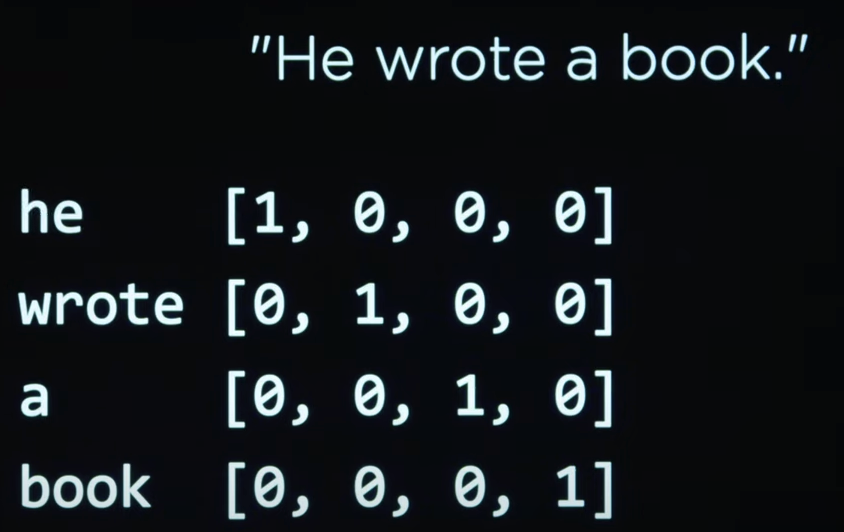
This is a very simple approach; however, simplicity comes at a cost. To represent each word in a text, we need a vector of size equal to the size of the vocabulary, which can be very large. Also, this approach does not capture the meaning of words and it does not take into account the context in which the words are used. Two words that have similar meanings will have totally different one-hot encodings.
Distributed Representation and Word Embeddings
To address the meaning problem, we can store words using real numbers, where each word is represented by a vector of real numbers and each element of the vector represents a feature of the word. Words with similar meanings will have vector values close to each other. This approach is called distributed representation. To generate these vectors, we can utilize machine learning models trained on large amounts of text data. Based on the context, the computer can learn words with similar or related meanings.
Word2vec
Word2Vec is a popular model for word distributional representation, developed by researchers at Google. It operates on the principle that words which appear in similar contexts often share similar meanings. Word2vec employs a shallow neural network to learn word representations from extensive text corpora.
Watch this video to delve deeper into word representation and Word2vec:
I'm blown away by the king-queen example in the above video. It's amazing how word2vec can capture the meaning of words.
The code utilized in the video is available here
Word Embeddings
Word embedding, a form of distributed representation, captures semantic relationships between words by mapping them to dense, low-dimensional vectors within a continuous vector space. Word2Vec serves as a specific algorithm for word embedding.
✅ Try this interesting tool to experiment with word embeddings. Clicking on one word reveals clusters of similar words: 'toy' clusters with 'Disney', 'LEGO', 'PlayStation', and 'console'.
Here's a Python example for word embedding:
from gensim.models import Word2Vec
from nltk.tokenize import word_tokenize
import nltk
nltk.download('punkt')

# Example sentences
sentences = [
    "The quick brown fox jumps over the lazy dog.",
    "The cat is cute.",
    "The dog is friendly."
]


# Tokenize the sentences
tokenized_sentences = [word_tokenize(sentence.lower()) for sentence in sentences]

# Train the Word2Vec model
model = Word2Vec(sentences=tokenized_sentences, vector_size=100, window=5, min_count=1, workers=4)

# Get the word vectors
word_vectors = model.wv

# Print the word vector for a specific word
print("Vector representation of 'dog':", word_vectors['dog'])

# Find similar words
similar_words = word_vectors.most_similar('dog')
print("Words similar to 'dog':", similar_words)
Bag-of-Words
Bag-of-Words (BoW) is a simple and popular method for representing text data. It is based on the idea that the order of words in a document does not matter, and that the presence of words in a document is more important than the order of the words. In our previous section when we talked about cleaning text by removing stop words and punctuation, we were preparing the text for BoW.
BoW represents a document as a vector of word counts. Each element in the vector represents the count of a word in the document. The size of the vector is equal to the size of the vocabulary. Here's an example of how to use BoW in nltk:
from sklearn.feature_extraction.text import CountVectorizer
corpus = [
    'This is the first document.',
    'This document is the second document.',
    'And this is the third one.',
    'Is this the first document?',
]
vectorizer = CountVectorizer()
X = vectorizer.fit_transform(corpus)
print(vectorizer.get_feature_names_out())
print(X.toarray())
The output of this code will be:
['and' 'document' 'first' 'is' 'one' 'second' 'the' 'third' 'this']
[[0 1 1 1 0 0 1 0 1]
 [0 2 0 1 0 1 1 0 1]
 [1 0 0 1 1 0 1 1 1]
 [0 1 1 1 0 0 1 0 1]
]
In the above sample, we can see that the word "document" appears once in the first document (first text in the corpus list), twice in the second document, 0 times in the third, and once in the fourth.
Document-Term Matrix (DTM):
DTM represents documents as rows and words (terms) as columns in a matrix. Each cell in the matrix represents the frequency of a particular word in a particular document.
This format is called the document-term matrix. Each row in the matrix represents a document, and each column represents a word in the vocabulary. The value in each cell represents the count of the word in the document. The document-term matrix can be used as input to machine learning models for tasks such as text classification, topic modeling, and sentiment analysis.
For example, if we have three documents ["The cat is cute.", "The dog is cute too.", "The cat and the dog are friends."], and a vocabulary of ["the", "cat", "is", "cute", "dog", "too", "and", "are", "friends"], the DTM might look like:
| the | cat | is | cute | dog | too | and | are | friends | |
|---|---|---|---|---|---|---|---|---|---|
| Doc1 | 1 | 1 | 1 | 1 | 0 | 0 | 0 | 0 | 0 |
| Doc2 | 1 | 0 | 1 | 1 | 1 | 1 | 0 | 0 | 0 |
| Doc3 | 2 | 1 | 1 | 0 | 1 | 0 | 1 | 1 | 1 |
Comparison
Each of the above techniques has its own advantages and disadvantages, and the choice of representation depends on the specific task at hand. Let's summarize the differences between word embedding, DTM, and BoW:
Word Embedding:
Represents words as dense vectors in a continuous vector space, capturing semantic similarities. Advantages:
- Captures semantic relationships between words effectively.
- Handles out-of-vocabulary words by learning continuous representations.
- Useful for various NLP tasks like classification, sentiment analysis, and translation.
Disadvantages:
- Requires substantial training data and computational resources.
- May struggle with rare or domain-specific words.
Suitable for tasks like sentiment analysis, language translation, and document clustering.
Document-Term Matrix (DTM):
Represents term frequencies in documents as a matrix, with rows for documents and columns for terms. Advantages:
- Provides a simple and interpretable representation of text data.
- Easy to implement and understand.
- Compatible with various machine learning algorithms. Disadvantages:
- Doesn't capture semantic relationships between words.
- Memory-intensive for large datasets due to high dimensionality.
Suitable for sentiment analysis, topic modeling, and spam detection.
Bag of Words (BoW):
The Bag of Words (BoW) model represents documents as unordered collections of word frequencies.
Advantages:
- Simple and intuitive representation of text data.
- Easy to implement and understand.
- Compatible with various machine learning algorithms. Disadvantages:
- Loses information about word order and context.
- Doesn't capture semantic relationships between words.
- Memory-intensive for large datasets due to high dimensionality.
Use Cases
-
One-hot Encoding:
- Typically used in tasks where categorical data, such as words or features, need to be represented as numerical vectors.
- Commonly employed in simple classification tasks or as input to machine learning models that require numerical inputs.
-
Distributed Representation and Word Embeddings (Word2Vec):
- Widely utilized in natural language processing (NLP) tasks to capture semantic relationships between words.
- Suitable for tasks like sentiment analysis, language translation, and document clustering.
- Especially effective in scenarios where contextual understanding and semantic relationships are crucial.
-
Bag-of-Words (BoW):
- Frequently used in text classification tasks where word order is not important.
- Suitable for sentiment analysis, topic modeling, and spam detection.
- Often applied in scenarios where the presence of specific words matters more than their sequence.
-
Document-Term Matrix (DTM):
- Commonly used in text mining and information retrieval tasks.
- Ideal for tasks like document clustering, keyword extraction, and topic modeling.
- Effective in scenarios where understanding the frequency distribution of words across documents is essential.
Summary
In this lesson, we explored key techniques for representing text in Natural Language Processing (NLP), covering one-hot encoding, Word2Vec, Bag-of-Words (BoW), and Document-Term Matrix (DTM). Each method offers unique strengths for tasks like text classification, sentiment analysis, and topic modeling. Understanding these techniques is essential for effective text analysis in NLP applications.
Practice: Data Cleaning
Follow the Colab notebook provided below to practice data cleaning:

Practice : Text Summarization
Follow the Colab notebook provided below to practice and build a text summarizer:

Language Models
Before we begin discussing language models, I'd like you to take a minute and think about the term "model." What does it mean to you? What comes to mind when you hear the word "model"? How useful do you find having a model of something?
What is a Model?
Not just yet. Take another minute and think more deeply about it.Click here to see the answer
When I hear the word "model," I usually think of a representation of something. It could be a physical representation, such as a miniature model of a building, or a conceptual representation, like a mathematical model of a system.Models help us make sense of the world around us by capturing the essential features of a system and abstracting away the details that are not relevant to the problem at hand. This approach enables us to better understand the dynamics of the system, focus on the important factors, and perform various operations on it.
What is a Language Model?
A language model is a representation of a language. We are interested in finding ways to represent languages so that machines can understand and process them.
One model I thought of while writing this section is one that represents sentences without any stop words or punctuation, with each word converted to its root form. How could this be useful? Well, this model could be used to compare sentences to see if they are similar or not, and perhaps even to compress text.
In the field of natural language processing (NLP), however, we are interested in more sophisticated models that can capture the entirety of a language and its dynamics. This helps us perform complex tasks such as machine translation, text summarization, and question answering.
Rule-based Language Models
The natural starting point for developing language models is to turn to the field of linguistics, which has been the study of languages for centuries. This involves understanding how linguists have defined and represented languages over time.
A common method in this area mirrors how we typically learn languages in school. We study grammar rules, vocabulary, and syntax. We learn to construct sentences, use punctuation, and spell words correctly. This approach to language learning is rule-based.
Grammar and Syntax
One method of teaching a computer to understand the structure of a natural language involves teaching it the rules of grammar and syntax. This constitutes the rule-based approach to language understanding.
A formal grammar is a collection of rules for generating sentences in a language.
A context-free grammar (CFG) is a type of formal grammar that describes the syntactic structure of a language through a set of production rules. These rules dictate how various constituents (such as words, phrases, and sentences) can be combined to form grammatically correct sentences. A context-free grammar includes the following elements:
Terminals: These are the basic building blocks of the language, including words or punctuation symbols. Terminals are the most fundamental units of the language and cannot be broken down further. For instance, in English, terms like "cat", "dog", "run", and "jump" serve as terminals.
Non-terminals: These symbols represent categories of linguistic elements, such as noun phrases (NP), verb phrases (VP), Nouns (N), and verbs (V), among others. Non-terminals act as placeholders that can be substituted with terminals or other non-terminals in accordance with the production rules.
Production Rules: These rules outline how non-terminals can be expanded or substituted by other symbols (terminals or non-terminals). Each rule includes a non-terminal symbol on the left-hand side and a sequence of symbols (terminals or non-terminals) on the right-hand side.
To delve deeper into context-free grammars and their application in sentence generation, watch this informative video:
The code sample below utilizes the Natural Language Toolkit (NLTK) library in Python to establish a context-free grammar (CFG) and parse sentences based on that grammar.
import nltk

# Define a context-free grammar (CFG) for parsing sentences
grammar = nltk.CFG.fromstring("""
    S -> NP VP

    AP -> A | A AP
    NP -> N | D NP | AP NP | N PP
    PP -> P NP
    VP -> V | V NP | V NP PP

    A -> "big" | "blue" | "small" | "dry" | "wide"
    D -> "the" | "a" | "an"
    N -> "she" | "city" | "car" | "street" | "dog" | "binoculars"
    P -> "on" | "over" | "before" | "below" | "with"
    V -> "saw" | "walked"
""")

# Create a parser using the defined grammar
parser = nltk.ChartParser(grammar)

# Take an input sentence from the user
sentence = input("Sentence: ").split()
try:
    # Parse the sentence and generate parse trees
    for tree in parser.parse(sentence):
        tree.pretty_print()
except ValueError:
    # If no parse tree is possible, inform the user
    print("No parse tree possible.")
In this approach, we manually feed the computer with the rules of grammar and syntax. This method, however, has its limitations, as it is challenging to formulate rules that cover all possible sentences in a language. Additionally, accounting for the inherent ambiguity of human language poses a significant challenge.
Statistical Language Models
You might already have an idea of what this entails. Isn't it similar to the approach we've been discussing throughout this course? We either hard-code the rules or—what's the other option? Yes, we use data to learn the rules or identify patterns.
Statistical language models are predicated on the notion that language behaves as a statistical phenomenon. These models employ statistical techniques to discern patterns and structures within a language from a vast corpus of textual data.
In statistical language models, rather than handling the entirety of the text data at once, we can adopt the n-gram methodology we explored earlier. This strategy involves segmenting the text into smaller fragments to learn patterns within each segment. This forms the basis of statistical language models. For instance:
Consider the sentence "I am going to the ". A statistical language model might predict that the next word is "store" with considerable probability because the phrase "going to the store" frequently occurs in English.
Or take the sentence "no the dark eat banana." A statistical language model could indicate that this sequence is likely not a valid English sentence. It might even suggest a more grammatically correct version of the sentence if possible.
Here's an interesting example involving the use of a Markov chain statistical model to generate text:
The code used in the video is available here
A Markov chain represents a mathematical model that transitions from one state to another among a finite or countable number of possible states.
Watch this video for a slightly different take on statistical language models:
Neural-Networks-based Language Models
Another approach to language modeling leverages neural networks to model the probability distribution over words in a sentence. Beyond this, we can employ various types of neural networks to learn different aspects, capture distinct patterns, and address a wide array of problems.
Watch this video to learn about neural network-based language models and how RNNs and Transformers are used in language modeling:
Recurrent Neural Networks (RNNs)
One of the most favored neural network architectures for language modeling is the Recurrent Neural Network (RNN). Designed to process sequential data, such as word sequences in a sentence, RNNs are adept at capturing the context of a word within its sentence, rendering them particularly suitable for language modeling tasks.
An advancement in language models involves the application of RNNs, especially Long Short-Term Memory (LSTM) networks, to model the probability distribution across words. We have a practice on this topic in the next section.
Transformers
The inherent sequential nature of RNNs introduces inefficiencies when processing lengthy data sequences, such as extended sentences or documents. This inefficiency stems from the vanishing gradient problem, hindering the network's ability to recognize long-range dependencies within the data. In response, researchers have devised more sophisticated neural network architectures like transformers, optimized for efficiently handling long data sequences.
Transformers employ the attention mechanism, enabling the model to concentrate on different segments of the input sequence during prediction. This model has attained unparalleled performance, forming the backbone of the most advanced language models, including BERT, GPT-2, and GPT-3.
Large Language Models
A "large" language model is typically characterized by its training on a vast dataset. The term "large" reflects not just the dataset's volume but also its complexity and diversity. These models are developed on extensive text corpora, potentially comprising billions or even trillions of words, gathered from a variety of sources like books, articles, websites, and other text repositories. Training on such broad datasets allows the model to acquire a comprehensive understanding of natural language, encompassing syntax, semantics, and contextual subtleties, often resulting in more accurate and robust models capable of efficiently performing a plethora of natural language processing tasks.
Training large language models requires considerable computational resources, such as powerful GPUs or TPUs, alongside expansive distributed training infrastructure. This process usually involves executing millions of iterations of the training algorithm, tuning the model parameters based on the gradients of the loss function relative to the parameters.
Language Models Examples
Modern language models such as Google's BERT, OpenAI's GPT series, Facebook AI's RoBERTa, and Palm's T5 signify progress in natural language processing.
BERT revolutionized understanding bidirectional context through its transformer architecture, enhancing performance in tasks like text classification and named entity recognition.
The GPT series, notably GPT-3, is celebrated for its autoregressive approach, sequentially generating coherent text based on preceding tokens. RoBERTa refined BERT's architecture, enhancing pre-training methods for better efficacy in tasks such as sentiment analysis and machine translation.
T5 marked a significant advancement by treating all NLP tasks as text-to-text tasks, thus enabling a unified approach to handling diverse tasks and facilitating adaptation to new domains. T5's adaptability, scalability, and its integration of transformer architecture with a multi-task learning approach, establish it as a cutting-edge solution for a broad range of language processing challenges.
Large Language Models Resources
For those keen on delving deeper into large language models, the following resources are invaluable:
- Large Language Models From Scratch
- How to Train a new Language Model
- How to Build a Large Language Model from Scratch Using Python
- Creating a Large Language Model from scratch: A beginner's guide
- GPT-3: Language Models are Few-Shot Learners
- BERT: Pre-training of Deep Bidirectional Transformers for Language Understanding
- T5: Exploring the Limits of Transfer Learning with a Unified Text-to-Text Transformer
Practice: Create Poetry
Carefully watch the video below and follow the associated Colab notebook to learn how to generate text using an LSTM:
Colab Notebook

Deep Reinforcement Learning for Dialogue Generation
This lesson is about the paper "Deep Reinforcement Learning for Dialogue Generation" by Jiwei Li, Will Monroe, Alan Ritter, Dan Jurafsky, Michel Galley, and Jianfeng Gao.
The paper was presented at the 2016 Conference on Empirical Methods in Natural Language Processing (EMNLP). The paper introduces a novel approach to dialogue generation using deep reinforcement learning, aiming to improve the quality and coherence of conversational agents.
The authors propose a model that combines reinforcement learning with sequence-to-sequence models to generate more contextually relevant and engaging responses. Through this lesson, students will learn about the challenges of dialogue generation and how deep reinforcement learning can be used to enhance the performance of conversational agents.
Read the paper here.
Happy learning!
Week 8 Quiz
Before attempting the quiz, read the following carefully.
- This is a timed quiz. You will have only one attempt.
- You will have 20 minutes to complete multiple-choice questions.
➡️ Access the quiz on here
Assignment : Next Word Prediction
Follow the below Colab notebook to complete the assignment on next word prediction:

Submission
Submit your assignment via gradescope here
Final Project
The final project is an opportunity for you to apply the knowledge and skills that you have learned in the course to a real-world problem. You are required to select one of the provided project ideas, develop a working solution, and submit 3 key deliverables:
- Working Project: A functional AI-based system.
- Source Code: The source code of the project (Github link).
- Project Report: A document detailing your development process, including the sections below.
Team Size: 1 - 3
Submission Deadline: 14 June 2024 Submission Link: Submit Your Project
Progressive Project Report
You are required to fill the project report progressively while working during week 9 and week 10. Otherwise, your submission might not be accepted. Progressively means that you should fill the report as you work on the project, not all at once at the end of the project.
Project Report
Your project report (a sample can be found here.) must document the following steps:
- Problem Identification: Clearly define your project's computational problem (~50 words).
- Exploration of Alternatives: Investigate various algorithms and methodologies that could solve the problem. Discuss the pros and - cons of at least three approaches (~200 words).
- Selection and Justification: Choose the most appropriate solution and provide a rationale for your choice based on its - efficiency, accuracy, and suitability for the problem (~50 words).
- Implementation Details: Provide details on the dataset used, the model/algorithm chosen, the frameworks and tools, etc.
- Demo Link: Include a link to a working demo of the project. It could be a live link on the web or a recorded video.
Project Ideas
Project 1: AI-Powered Home Security System
Objective: Develop a system that utilizes cameras placed at home entrances to detect and alert homeowners about human presence in a designated security zone. Requirements: Implement an object detection system to identify human figures in a video feed.
Project 2: Stock Market Prediction
Objective: Construct a model to forecast future stock prices using historical data.
Requirements: Develop a time series forecasting model that predicts the stock price of a certain company. Visualize prediction accuracy and model performance.
Project 3: Business Question Answering System
Objective: Build an AI-driven system that acts as a customer service agent to answer frequently asked questions about a business.
Requirements: Develop a natural language processing model capable of understanding and responding to user queries.
Evaluation Rubric
Problem Identification (10 Points)
- [0 Points]: The problem is not clearly defined; lacks detail.
- [3 Points]: The problem is identified but not clearly articulated; some details are missing.
- [5 Points]: The problem is well-defined and detailed with clear relevance to AI.
Methodology (20 Points)
- [20 Points]: Excellent, thorough exploration of varied alternatives; detailed analysis including pros and cons of each. Well-justified selection; reasoning is comprehensive, detailed, and thoroughly logical.
- [15 Points]: Moderate exploration of alternatives; moderate detail and consideration of options.
- [10 Points]: Some exploration of alternatives; moderate detail and consideration of options.
- [4 Points]: Limited or no exploration of alternative solutions; lacks depth.
Implementation and Testing (70 Points)
- [60-70 Points]: Excellent implementation; system functions flawlessly with reasonable performance and robust testing. Process and implementation details well documented.
- [50-60 Points]: Good implementation; system functions as intended with good performance. Documentation is adequate.
- [40-50 Points]: Implementation is mostly complete; minor issues in functionality or performance.
- [0-40 Points]: Implementation is incomplete or flawed; major issues in functionality.
Total Points: 100