Regression Evaluation Techniques
In previous lessons, we've seen how we can evaluate ML classification models to ascertain its performance and generalization capability to new and unseen data. Now we want to look at how we can evaluate our regression models which deals with continuos variable (i.e., numbers), unlike classification that deals with categorical data. Without proper evaluation, we cannot determine how well the model is performing or how accurate its predictions are.
Regression evaluation
Regression evaluation techniques are methods used to assess the performance of regression models. They can be used to determine how well the model fits the training data, how well it generalizes to new data, and how accurate its predictions are. There are a number of different regression evaluation techniques, but some of the most common include:
- Mean Absolute Error
- Mean Squared Error
- Root Mean Absolute Error
- R-squared (R²)
To understand these metrics, let's use a sample regression model. Suppose we have a regression model that can predict air pollution levels (measured in Particulate Matter 2.5 - PM2.5) in a city based on weather conditions and traffic data. We have a dataset with 10 actual air pollution values (in micrograms per cubic meter or µg/m3) and their corresponding predicted values obtained from our regression model.
- Actual PM2.5 values:
[20, 25, 30, 35, 40, 45, 50, 55, 60, 65] - Predicted PM2.5 values:
[18, 24, 32, 38, 43, 47, 52, 57, 62, 68]
To know if our model is accurate in predicting air pollution, we can evaluate the model using the metrics listed above.
Mean Absolute Error (MAE)
MAE measures the average absolute difference between the predicted values and the actual values. It gives us an idea of how far off, on average, the predictions are from the true values. A lower MAE indicates better model performance. For example, if the MAE is 3, it means, on average, the model's predictions are off by 3 units from the actual values.
Using our pollution prediction model, we take the absolute difference between each predicted and actual value, sum them up, and then divide by the number of data points.
MAE = (|20-18| + |25-24| + |30-32| + ... + |60-62| + |65-68|) / 10
MAE = (2 + 1 + 2 + 3 + 3 + 2 + 0 + 2 + 2 + 3) / 10
MAE = 20 / 10
MAE = 2
This MAE indicates on average, the model's predictions are off by 2 µg/m3 from the actual values.
Mean Squared Error (MSE):
MSE measures the average squared difference between the predicted values and the actual values. MSE penalizes larger errors more heavily, which means it amplifies the impact of outliers. A lower MSE indicates better model performance. For example, if the MSE is 9, it means, on average, the model's predictions are off by 9 units squared from the actual values.
Using our pollution prediction model, we take the square of the difference between each predicted and actual value, sum them up, and then divide by the number of data points.
MSE = ((20-18)^2 + (25-24)^2 + (30-32)^2 + ... + (60-62)^2 + (65-68)^2) / 10
MSE = (4 + 1 + 4 + 9 + 9 + 4 + 0 + 4 + 4 + 9) / 10
MSE = 44 / 10
MSE = 4.4
This MSE indicates on average, the model's predictions are off by 4.4 µg/m3 squared from the actual values.
Root Mean Squared Error (RMSE):
RMSE is the square root of MSE and gives us a measure of the average difference between predicted and actual values in the same units as the target variable.
Using our pollution prediction model, we can calculate the RMSE as follows:
RMSE = √(MSE)
RMSE = √(4.4) ≈ 2.10
R-squared (R²):
R², also known as the coefficient of determination, measures how well the model's predictions explain the variations in the data. It provides a value between 0 and 1, where 0 means the model does not explain any variation, and 1 means the model perfectly explains all the variations in the data. A higher R-squared value indicates better model performance. For example, an R-squared value of 0.75 means the model can explain 75% of the variations in the data.
Using our pollution prediction model, R² is calculated as the ratio of the variance explained by the model to the total variance of the data.
R² = 1 - (MSE of the model / MSE of the mean)
R² = 1 - (4.4 / ((20-20.5)^2 + (25-20.5)^2 + ... + (65-20.5)^2) / 10)
R² ≈ 0.76
This R² means the model can explain 76% of the variations in the data.
Reveal answer - regression techniques
Mean Absolute Error (MAE):
MAE = (|250-255| + |300-305| + |350-345| + ... + |550-560| + |600-610|) / 8
MAE = (5 + 5 + 5 + 10 + 5 + 5 + 10 + 10) / 8
MAE = 55 / 8
MAE ≈ 6.88
Mean Squared Error (MSE):
MSE = ((250-255)^2 + (300-305)^2 + (350-345)^2 + ... + (550-560)^2 + (600-610)^2) / 8
MSE = (25 + 25 + 25 + 100 + 25 + 25 + 100 + 100) / 8
MSE = 425 / 8
MSE = 53.13
Root Mean Squared Error (RMSE):
RMSE = √(MSE) = √(53.13) ≈ 7.29
R-squared (R²):
R-squared = 1 - (53.13 / ((250-425)^2 + (300-425)^2 + ... + (600-425)^2) / 8)
R-squared ≈ 0.89
In this exercise, our model shows relatively low MAE and RMSE and a reasonably high R-squared, suggesting that it can predict housing prices with good accuracy.
Implementation of evaluation metrics
Now, let's look at developing a pollution prediction model and evaluating it using the metrics above. To develop this model, we'll use a simple example where we have actual pollution levels and their corresponding predicted values from the model. Let's assume we have the following data:
- Actual pollution levels:
[30, 40, 50, 60, 70, 80, 90, 100] - Predicted pollution levels:
[32, 38, 53, 62, 68, 78, 88, 96]
In this model implementation, we created a simple linear regression model using scikit-learn, fit it to the data, make predictions, and then calculate the evaluation metrics. The MAE, MSE, RMSE, and R-squared values will give us insights into the performance of the model in predicting pollution levels.
👩🏾🎨 Practice: Regression evaluation... 🎯
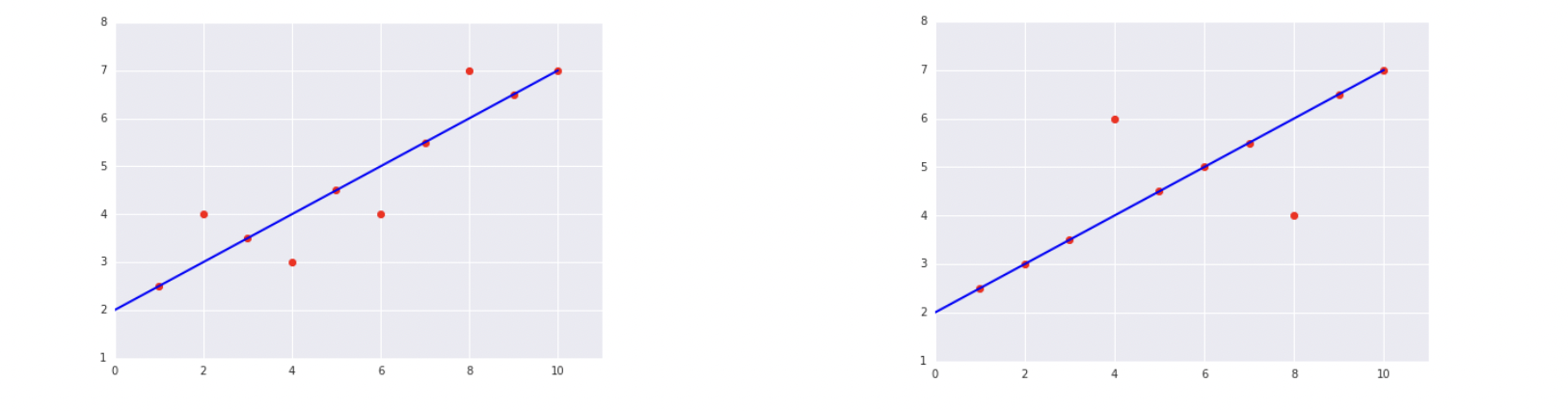
-
Which of the two data sets shown in the preceding plots has the higher Mean Squared Error (MSE)?
- The data on the right
- The data on the left
-
You are given a dataset containing information about houses, including their area, number of bedrooms, and the actual price. Your task is to evaluate a regression model that predicts house prices based on these features.
| Area (sq. ft.) | Bedrooms | Actual Price ($) | Predicted Price ($) |
|---|---|---|---|
| 1500 | 2 | 250000 | 240000 |
| 1800 | 3 | 300000 | 310000 |
| 1200 | 2 | 180000 | 175000 |
| 2200 | 4 | 400000 | 390000 |
| 1600 | 3 | 280000 | 265000 |
| 1400 | 2 | 220000 | 225000 |
| 2000 | 3 | 320000 | 330000 |
| 1700 | 3 | 270000 | 260000 |
| 1300 | 2 | 200000 | 205000 |
| 1900 | 3 | 310000 | 300000 |
- Calculate the MAE, MSE, and RMSE for the given dataset.
➡️ Next, we'll look at
Model selection... 🎯.